Chapter 3 answers the question every backend engineer should be able to answer in an interview: "How does a database actually store and retrieve data?" Kleppmann walks through two fundamentally different storage engine families, explains how indexes work, and then pivots to the analytical world of data warehouses and column stores.
- LSM-tree favors writes — sequential appends to memtable then flushed SSTables; Bloom filters skip unnecessary disk reads. Used by Cassandra, RocksDB, HBase.
- B-tree favors reads — one path root-to-leaf; in-place page updates with WAL for crash recovery. Used by PostgreSQL, MySQL/InnoDB, SQLite.
- Write-ahead log (WAL) — both B-trees and LSM-trees use a WAL for durability; B-tree WAL is for crash recovery of in-place writes; LSM-tree WAL recovers the unflushed memtable.
- Clustered vs non-clustered indexes — clustered stores row data inside the index leaf (InnoDB primary key); non-clustered stores a pointer to the heap file; a covering index includes extra columns to avoid the heap lookup entirely.
- OLTP vs OLAP are fundamentally different access patterns — OLTP: random small point queries; OLAP: full sequential scans over millions of rows. Run them on separate systems.
- Column-oriented storage — stores all values for one column together; reads only needed columns; compresses aggressively (bitmap, RLE, dictionary); enables CPU SIMD vectorized execution.
LSM-trees (log-structured) favor writes; B-trees favor reads. Both use indexes to make queries fast, with different tradeoffs. OLTP databases optimize for random-access point queries; OLAP warehouses optimize for sequential full-column scans. Column-oriented storage is the key insight that makes analytical queries fast.
Original Notes
The handwritten study notes this chapter summary is based on:
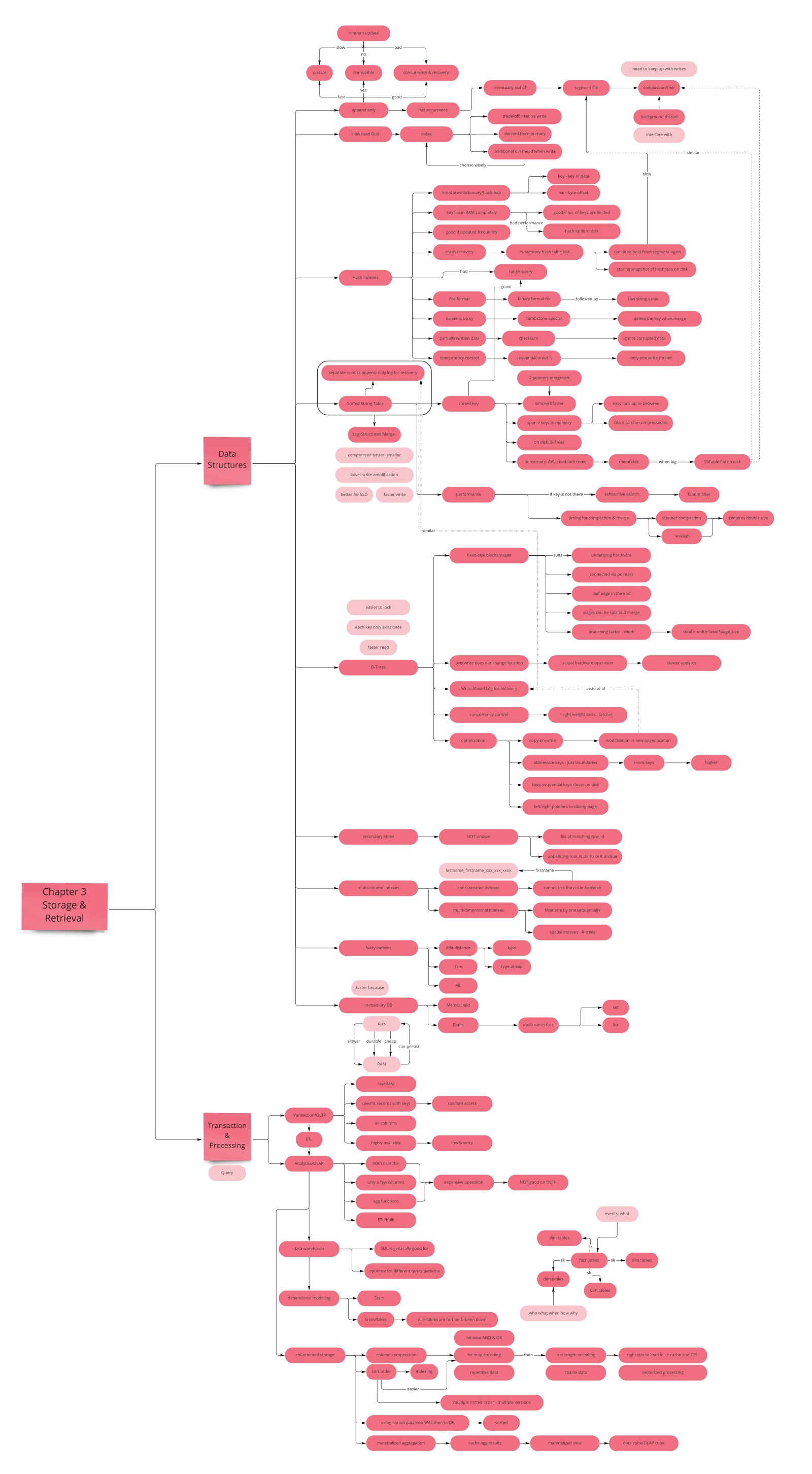
Log-Structured Storage Engines
Kleppmann builds intuition from the ground up, starting with the simplest possible "database" — two bash functions:
db_set() { echo "$1,$2" >> database; }   # append-only
db_get() { grep "^$1," database | tail -n1 | cut -d',' -f2; }
This "database" has O(1) writes (sequential append to a file — the fastest possible I/O) and O(n) reads (full scan to find the latest value). The append-only design is not a curiosity — it is the foundation of every log-structured storage engine. Appending to the end of a file is the most efficient disk operation: it never requires seeking backward, never creates fragmentation, and is crash-safe (a power failure during an append either writes the record or does not; it cannot corrupt previously written data). The read problem is what indexes solve.
Hash Index (Bitcask)
The hash index is the simplest index structure for an append-only log. Bitcask (the default storage engine in Riak) maintains an in-memory hash map from every key to the byte offset of its most recent value in the log file. Each write appends a new entry to the log and updates the in-memory hash map pointer. Each read performs one disk seek to the stored offset and loads the value. No scanning needed.
The critical constraint: the entire key set must fit in RAM. The values can be arbitrarily large and live on disk; only the keys and offsets need to be in memory. This constraint is acceptable for workloads with a bounded number of distinct keys but a high update rate per key — think URL shorteners (millions of URLs, each clicked and updated many times), IoT sensor readings (thousands of sensor IDs, millions of time-series values), or session stores (fixed user count, frequently refreshed sessions).
The log file grows without bound, so Bitcask segments the log into files of a maximum size. Compaction runs as a background process: it reads multiple segment files, keeps only the most recent value for each key (discarding all earlier values for the same key), and writes a new merged segment file. Old segment files are deleted once the merged file is written and the in-memory hash map is updated. Compaction runs concurrently — reads continue against the old segments while compaction writes the new one, then an atomic pointer swap transitions to the new segment.
On crash recovery, the in-memory hash map is lost. Bitcask rebuilds it by replaying the log on restart — but this is slow for large logs. The optimization is to write a hash map snapshot to disk periodically; on restart, load the snapshot and replay only the segment entries written since the last snapshot.
Three reasons. First, sequential writes are much faster than random writes on spinning disks, and still significantly faster on SSDs (which have write amplification and wear leveling characteristics that make random writes more expensive). Second, append-only makes concurrency simpler — there is no contention between writers updating the same location. Third, crash recovery is cleaner — a partially-written append is at the end of the file and can be detected and discarded; a partially-written in-place update leaves the record in an unknown state.
SSTables and the LSM-Tree
Sorted String Tables (SSTables) add one constraint to the append-only log segment: keys within each segment file must be sorted. This single constraint unlocks three powerful capabilities:
- Efficient merging: merging multiple segment files is exactly merge sort — read the first key from each file's sorted run, write the smallest to the output, advance. O(n) time, constant memory.
- Sparse in-memory index: because keys are sorted, you only need one in-memory index entry every few kilobytes. To find key "home," look up the sparse index to find that "hand" is at offset 1200 and "how" is at offset 1500 — then scan the 300 bytes in between. Much smaller memory footprint than one entry per key.
- Range queries: keys between "apple" and "banana" are physically adjacent in the sorted file — read the range sequentially instead of issuing separate lookups per key.
The Log-Structured Merge-Tree (LSM-Tree), described by Patrick O'Neil et al. in 1996 and popularized by LevelDB (Google), RocksDB (Meta/Facebook), Apache Cassandra, and Apache HBase, maintains SSTables through the following lifecycle:
- Writes go to the memtable — an in-memory balanced binary search tree (red-black tree or skip list) that keeps keys sorted at all times. Writes are always O(log n) in memory, extremely fast.
- WAL for durability — every write is first appended to a Write-Ahead Log on disk. If the process crashes before the memtable is flushed, the WAL is replayed on restart to reconstruct the memtable. The WAL is discarded once the memtable successfully flushes.
- Flush to SSTable — when the memtable exceeds a threshold (typically a few megabytes), it is written to disk as a new SSTable. Because the memtable is a sorted tree, the resulting SSTable is already sorted — no additional sort pass needed.
- Reads check in order: first the memtable (current writes), then the most recent on-disk SSTable, then progressively older SSTables. A key that was recently written will be found quickly; an old key may require checking multiple SSTables.
- Background compaction merges and garbage-collects SSTables, keeping disk space bounded and read performance acceptable by reducing the number of SSTables a read must check.
Bloom Filters: Avoiding Unnecessary Disk Reads
LSM-tree reads have a fundamental weakness: for a key that does not exist, the read must check the memtable and every SSTable (unless the key can be quickly eliminated). For write-heavy workloads with frequent negative lookups (e.g. checking whether a key exists before writing it), this is expensive. Bloom filters solve this.
A Bloom filter is a probabilistic data structure that uses a bit array and multiple hash functions. To add a key, compute k hash functions and set those k bits to 1. To query a key, compute the same k hash functions and check those k bits. If any bit is 0, the key is definitely not present (no false negatives). If all bits are 1, the key is probably present (false positives are possible but controlled by filter size). LSM-trees attach one Bloom filter per SSTable. When a read needs to check an SSTable, the Bloom filter is consulted first — if it says "definitely not here," the SSTable is skipped entirely, saving a disk read. In practice this dramatically reduces the read amplification for non-existent keys.
Compaction Strategies: Size-Tiered vs Leveled
Compaction is the background process that merges SSTables to reclaim disk space and reduce read amplification. Different compaction strategies make different tradeoffs:
| Strategy | How It Works | Write Amplification | Space Amplification | Used By |
|---|---|---|---|---|
| Size-tiered | Group similar-size SSTables; merge groups when a threshold count is reached | Lower — merges happen less frequently | Higher — during merge, old + new files coexist (up to 2× space temporarily) | Cassandra (default), HBase |
| Leveled | SSTables organized into levels; each level has a size limit; L0 is flushed from memtable; when a level is full, SSTables are merged into the next level | Higher — data is rewritten across levels | Lower — each key exists at most once per level (except L0) | LevelDB, RocksDB, Cassandra (option) |
Leveled compaction keeps total data size per level bounded, which means it uses disk space more efficiently and provides more predictable read performance (fewer levels to check). Size-tiered compaction produces fewer total writes, which is better for write-heavy workloads, but at the cost of higher space amplification during merges. RocksDB supports both strategies and allows tuning for the workload — this is why it is used in systems as different as MyRocks (MySQL on RocksDB), TiKV (distributed key-value store), and CockroachDB (distributed SQL).
B-Tree Storage Engines
B-trees are the dominant index structure for relational databases. PostgreSQL, MySQL/InnoDB, SQLite, Oracle, and SQL Server all use B-trees as their primary index structure. Understanding why requires understanding what problems B-trees were designed to solve and what invariants they maintain.
Structure and In-Place Updates
Unlike LSM-trees that break data into variable-length segment files, B-trees break the database into fixed-size pages or blocks, traditionally 4 KB — the same size as a disk sector, which enables efficient I/O. The tree is balanced: all leaf pages are at the same depth. Leaf pages contain actual key-value pairs (or references to heap file locations for non-clustered indexes). Internal pages (internal nodes) contain keys and pointers to child pages.
When you query a B-tree, you start at the root page, find the range that contains your key, follow the pointer to the appropriate child page, and repeat until you reach a leaf. This root-to-leaf traversal is O(log n) but with a very high branching factor — a B-tree of depth 3 with 4 KB pages and 4-byte keys can reference up to 256 TB of data. In practice, a B-tree depth of 3–4 is sufficient for most production databases, meaning most reads require 3–4 page reads (or fewer, since the upper levels are almost always cached in the buffer pool).
Writes update pages in place. To update a key's value, find the leaf page containing the key and overwrite the value in that page. If a new key is inserted and the leaf page is full, the page is split into two pages, and the parent page is updated to contain the new dividing key. This split can cascade upward if the parent is also full, in the worst case splitting all the way to the root and creating a new root, increasing tree height by one. B-trees are kept balanced through this splitting mechanism.
Write-Ahead Log (WAL / Redo Log)
In-place updates are dangerous: if a crash occurs mid-update (e.g. while a page split is in progress), the database could be left in an inconsistent state — the split page exists but the parent pointer has not been updated. B-trees solve this with a Write-Ahead Log (WAL), also called a redo log in some systems. Before modifying any page, the modification is written to an append-only WAL file on disk. If the system crashes, the WAL is replayed on restart to bring the database back to a consistent state.
The WAL is also used for replication in many systems (PostgreSQL's WAL streaming replication, MySQL's binary log). This dual-use is efficient but creates coupling between crash recovery and replication, which complicates some operational scenarios.
Write amplification is the ratio of bytes written to disk to bytes of application data written. A single key-value write that causes a 4 KB page to be written has a write amplification of (4096 / data_size). For B-trees, a small update forces writing an entire page. Compaction in LSM-trees causes data to be written multiple times across levels. High write amplification reduces write throughput and accelerates SSD wear. This is a key reason to choose LSM-trees for write-heavy workloads — sequential compaction writes are more SSD-friendly than random B-tree page updates.
LSM-Tree vs B-Tree: The Full Comparison
| Property | LSM-Tree | B-Tree |
|---|---|---|
| Write path | Sequential appends to memtable + WAL; periodic flush to SSTable; background compaction | Random in-place page updates + WAL entry per write; occasional page split |
| Write amplification | Lower for initial write; compaction rewrites data multiple times across levels | Higher per update (entire page written); worse on SSDs for random small writes |
| Read performance | Slower — may need to check memtable + multiple SSTables; Bloom filters mitigate for non-existent keys | Faster — deterministic O(log n) root-to-leaf path; upper levels always cached |
| Read amplification | Higher — multiple SSTables may need checking for one key | Lower — one path from root to leaf for any key |
| Space amplification | Higher during compaction (old + new data coexist); tombstones until compacted away | Lower — in-place updates; free pages reclaimed immediately by B-tree page allocator |
| Compression ratio | Better — sorted, sequential layout compresses well | Worse — random page layout with fragmentation from page splits |
| Write latency | More predictable (memtable writes) but compaction can cause latency spikes | Can spike during page splits; generally good for mixed workloads |
| Concurrency model | Simpler — SSTables are immutable once written; no concurrent modification | Complex — pages can be modified concurrently; requires careful latch (short-lock) management |
| Typical use cases | Write-heavy workloads, time-series, event logs, high-volume IoT data ingestion | Read-heavy or mixed OLTP; queries that require strong read latency guarantees |
| Example systems | Cassandra, RocksDB, HBase, LevelDB, ScyllaDB | PostgreSQL, MySQL/InnoDB, SQLite, Oracle, SQL Server |
The comparison is not simply "LSM for writes, B-tree for reads." Real workloads are mixed, and the choice depends on write-to-read ratio, key distribution, disk type (SSD vs HDD), latency requirements, and operational complexity tolerance. Many modern systems mix both: RocksDB (LSM) is used as the storage engine under MySQL (MyRocks) to improve write throughput on SSD, while keeping MySQL's SQL interface. CockroachDB uses RocksDB internally while exposing full SQL with ACID transactions.
Index Structures Beyond the Primary Key
Secondary Indexes
The primary index maps a primary key to a row — by definition unique per row. A secondary index maps values of some other column (or combination of columns) to the rows that have that value. Both B-trees and LSM-trees can serve secondary indexes; the data structure is the same, but the key type differs.
The critical distinction: secondary index values are not unique. An index on city_id may map one city ID to millions of user rows. Each index entry points to a list (or a key range) of matching rows rather than a single row. This is implemented either by including the primary key in each secondary index entry (so the full row is fetched via a second primary key lookup) or by pointing directly to the heap file location (which becomes stale if the row moves, requiring careful maintenance).
Secondary indexes are essential for query performance — without them, any query filtering on a non-primary-key column requires a full table scan. Adding a secondary index dramatically speeds up reads at the cost of write overhead (every insert or update must also update all secondary indexes) and storage space. The tradeoff is explicit and measurable, which is why database schema design involves deliberate decisions about which secondary indexes to create.
Clustered vs Non-Clustered vs Covering Indexes
These three concepts are among the most commonly asked-about indexing details in database performance discussions and system design interviews.
In a clustered index, the actual row data is physically stored inside the index structure itself — specifically inside the leaf pages of the B-tree. InnoDB (MySQL's default storage engine) always uses the primary key as a clustered index: the primary key B-tree is the table itself. Looking up a row by primary key is a single tree traversal that delivers the full row. There can be only one clustered index per table (because the data can only be physically sorted in one way).
In a non-clustered index (also called a heap file index), the index stores a key-pointer pair: the indexed column value alongside a pointer to the row's location in a separate heap file. Lookups by the indexed column find the pointer, then perform a second I/O to the heap file to fetch the full row. This is a "double lookup" — two disk reads where a clustered index needs one. The heap file pointer can also become stale if the row moves (e.g. during a page compaction), requiring the index to be updated.
A covering index (or index-only scan) is an optimization: add extra columns to a secondary index beyond the indexed key so that a query can be answered entirely from the index without touching the heap at all. If your most frequent query is SELECT name, email FROM users WHERE city_id = 42, creating an index on (city_id, name, email) allows the query engine to satisfy the query entirely from the index. The "covered" columns are stored redundantly (they also exist in the heap), but the read is faster because the heap I/O is eliminated.
-- Non-clustered index: index on city_id, heap lookup to get name + email
CREATE INDEX idx_city ON users(city_id);
-- Read path: city_id B-tree → heap file lookup (2 I/Os)

-- Covering index: index includes name + email; no heap lookup needed
CREATE INDEX idx_city_cover ON users(city_id, name, email);
-- Read path: city_id B-tree only, name+email served from index leaf (1 I/O)

-- PostgreSQL: EXPLAIN output for index-only scan
EXPLAIN SELECT name, email FROM users WHERE city_id = 42;
--  Index Only Scan using idx_city_cover on users
--    Index Cond: (city_id = 42)
Multi-Column and Fuzzy Indexes
A multi-column index (composite index) covers multiple columns. The index is sorted first by the leading column, then by subsequent columns within each leading column group. The query WHERE last_name = 'Smith' AND first_name = 'John' can use a composite index on (last_name, first_name) very efficiently — it is a single sorted range lookup. However, the query WHERE first_name = 'John' alone cannot use that index efficiently (the leading column is missing) — it would require a full index scan. The column order in a composite index matters, and the right order depends on your query patterns.
Standard B-tree indexes are efficient for exact-match and range queries on structured data. They are not suitable for full-text search (which requires understanding word stemming, synonyms, typos) or approximate queries. Inverted indexes (like those used by Elasticsearch and Lucene) handle full-text search: they map each word to the list of documents containing that word, enabling efficient term-at-a-time scoring and Boolean combinations. For fuzzy matching (finding strings within a Levenshtein edit distance of k), specialized structures like BK-trees or SimHash are used. The key lesson: the right index structure depends entirely on the query type, not just on the data type.
In-Memory Databases
All disk-based storage engines — B-tree and LSM-tree alike — incur the cost of encoding application data structures into a format that can be stored on disk and decoded back on read. In-memory databases sidestep this entirely: the authoritative dataset lives in RAM, and the full richness of in-memory data structures (hash tables, skip lists, priority queues, trees) is available without serialization overhead.
Common examples: Redis (key-value, list, set, sorted set, hash, stream — all in memory with optional persistence), Memcached (pure cache, no persistence), VoltDB (ACID-transactional relational in-memory), MemSQL/SingleStore (in-memory with disk-backed durability), and Hazelcast (distributed in-memory data grid).
Kleppmann makes an important point that is often misunderstood: the performance advantage of in-memory databases is not primarily because they avoid disk reads — a well-configured disk-based database's working set fits in its buffer pool and rarely touches disk anyway. The advantage is that they avoid the overhead of encoding and decoding data structures into disk-friendly formats. An in-memory database can store a Redis sorted set as a real skip list with real pointers; a disk-based system would need to serialize and deserialize it on every access. The resulting code is also often faster because the in-memory data structures can be more complex and efficient than their serializable equivalents.
Durability for in-memory databases comes from periodic snapshots to disk (Redis RDB), append-only operation logs (Redis AOF), synchronous replication to other nodes (VoltDB), or NVM (non-volatile memory) hardware. The "restart and reload" time is a real operational concern — a Redis instance with 100 GB of data may take minutes to reload from disk after a restart, during which it is unavailable.
OLTP vs OLAP: Two Different Worlds
Online Transaction Processing (OLTP) and Online Analytical Processing (OLAP) represent fundamentally different usage patterns that have driven different storage architectures. Understanding both — and why they are kept separate — is one of the most important concepts in data engineering.
| Property | OLTP | OLAP |
|---|---|---|
| Primary user | End-users, via application | Data analysts, data scientists, business intelligence tools |
| Query pattern | Point lookups and small updates; "what is the order status for order #12345?" | Aggregations over millions of rows; "what was total revenue by region last quarter?" |
| Data touched per query | Tens to hundreds of rows | Millions to billions of rows |
| Bottleneck | Latency — must respond in milliseconds; concurrent user load | Throughput — must scan vast data efficiently; query complexity |
| Write pattern | Random, low-latency individual row inserts/updates | Bulk ETL loads, event stream ingestion — high volume, often batch |
| Dataset size | GB to TB | TB to PB |
| Schema | Normalized, third normal form or higher | Denormalized, star or snowflake schema optimized for query performance |
| Indexes | B-trees, secondary indexes on frequently filtered columns | Column-oriented storage; bitmap indexes; minimal row-level indexes |
| Example systems | PostgreSQL, MySQL, Oracle, SQL Server | Amazon Redshift, Google BigQuery, Snowflake, Clickhouse, Apache Druid |
The reason organizations run separate systems is that optimizing for one access pattern actively harms performance for the other. Running analytical queries on an OLTP database takes up connection pool slots, causes buffer pool thrashing (analytics scans displace the OLTP working set from cache), and contends for CPU and I/O with latency-sensitive transactional queries. Conversely, the highly normalized schemas and row-oriented storage of OLTP systems are poorly suited to analytical aggregations across millions of rows.
Data Warehouses and the ETL Pipeline
A data warehouse is a separate read-optimized analytical database, loaded from OLTP systems on a regular schedule via an ETL (Extract, Transform, Load) pipeline. The extract step pulls data from operational systems (often via database replication or change data capture). The transform step cleans, normalizes, and reshapes data into the warehouse's schema. The load step inserts the data into the warehouse.
ETL runs on a schedule (nightly, hourly, or near-real-time) rather than synchronously with OLTP writes, introducing a propagation delay. A sale made at 11:59 PM might not appear in the warehouse until after the nightly ETL completes. Modern "streaming ETL" architectures (using Kafka, Flink, or Spark Streaming) reduce this lag to seconds or minutes, enabling near-real-time analytics, but add architectural complexity.
The data warehouse exposes a SQL interface that is surface-level similar to OLTP SQL, but the underlying execution engine is radically different — built for massive parallel scans rather than indexed point lookups. SQL analysts who write against the warehouse do not need to understand this distinction; the declarative query interface hides it. This is one of the great practical successes of the declarative query model.
Star Schema and Snowflake Schema
The dominant schema pattern in data warehouses is the star schema. At its center is a fact table, where each row represents an event: a sale, a click, a page view, a login, an ad impression. Fact tables are typically the largest tables in the warehouse — billions of rows, each representing one occurrence of a business event. Each row contains foreign keys to multiple dimension tables (product, customer, date, store, geography, campaign) and one or more numeric measures (amount, quantity, duration, revenue).
-- Star schema: fact table at center, dimensions radiating out
CREATE TABLE fact_sales (
  sale_id       BIGINT,
  date_key      INT,        -- FK → dim_date
  product_key   INT,        -- FK → dim_product
  customer_key  INT,        -- FK → dim_customer
  store_key     INT,        -- FK → dim_store
  quantity      INT,
  amount_cents  BIGINT
);

-- Typical OLAP query: aggregation across millions of rows, few columns
SELECT d.month, p.category, SUM(f.amount_cents) AS revenue
FROM fact_sales f
  JOIN dim_date d     ON f.date_key    = d.date_key
  JOIN dim_product p  ON f.product_key = p.product_key
WHERE d.year = 2024 AND p.category = 'Electronics'
GROUP BY d.month, p.category
ORDER BY d.month;
The snowflake schema is a variant where dimension tables are further normalized into sub-dimensions. For example, instead of a flat dim_product table with category_name as a text column, a snowflake schema has a dim_product table with a foreign key to a separate dim_category table. Snowflake schemas are more normalized (less redundancy, smaller storage), but they require more joins per query. Most analytical query engines prefer star schemas for this reason — fewer joins, simpler query planning, and better query performance.
Column-Oriented Storage
The most important storage insight for analytical systems is column-oriented storage — and understanding why it matters requires understanding the I/O pattern of analytical queries. Consider a fact table with 100 columns and 1 billion rows. A typical OLAP query touches perhaps 3–5 of those columns but must scan all 1 billion rows for those columns. In row-oriented storage (PostgreSQL, MySQL), data is laid out as: all columns of row 1, then all columns of row 2, etc. To read 3 columns for 1 billion rows, you must load all 100 columns of all 1 billion rows from disk — reading 97% of data you do not need.
In column-oriented storage (Redshift, Snowflake, ClickHouse, Vertica, Apache Parquet), data is laid out as: all values of column 1 for all rows, then all values of column 2 for all rows, etc. To read 3 columns for 1 billion rows, you load only those 3 columns — 3% of total data. The I/O reduction is approximately (columns needed / total columns). For a table with 100 columns and a query touching 4, this is a 25× reduction in I/O — a transformative improvement for disk-bound analytical workloads.
Column Compression
Column storage enables aggressive compression because each column contains values of the same type and often a small number of distinct values. Compression reduces both disk storage cost and the amount of data transferred from disk to CPU — further improving query performance. The main techniques:
- Bitmap encoding: for a column with low cardinality (few distinct values relative to row count), create one bit vector per distinct value, where bit i is 1 if row i has that value. A
product_categorycolumn with 50 distinct categories across 1 billion rows can be represented as 50 bit vectors of 1 billion bits each — roughly 6 GB total instead of ~4 GB of 4-byte integers. The real win: operations like filtering (WHERE category = 'Electronics') become bitwise AND operations on bit vectors, which modern CPUs execute extremely efficiently using SIMD instructions. - Run-length encoding (RLE): when data is sorted by the column, consecutive rows often have the same value. RLE represents a run of N identical values as the pair (value, N). A
store_idcolumn sorted by store might have runs of 10,000 rows all with the same store ID. Instead of storing 10,000 integers, you store one (store_id, 10000) pair. This can reduce storage by 100–1000× for highly repetitive sorted data, and it makes GROUP BY operations trivially fast (each run is one group). - Dictionary encoding: replace each distinct value with a small integer code; store a dictionary mapping codes to values; store the column as integer codes. For a
country_codecolumn with 200 distinct values, replace 2-byte strings with 1-byte codes. Dictionary encoding is used by Parquet, ORC, and most columnar formats. It also enables predicate pushdown:WHERE country = 'US'becomes a lookup in the dictionary (find code for 'US'), then a simple integer comparison — no string parsing per row.
Vectorized Processing
Compression enables a further optimization: vectorized execution (also called SIMD vectorized processing). Modern CPUs have SIMD (Single Instruction Multiple Data) instruction sets (SSE, AVX, AVX-512) that operate on vectors of values simultaneously — for example, a single AVX-512 instruction can compare 16 32-bit integers against a constant in one CPU cycle. Columnar storage with compressed integer codes feeds directly into SIMD operations: a bitmap column can be ANDed with another in one instruction per 64 rows. Row-based storage, by contrast, requires branching on the column type at each row, preventing SIMD optimization.
The combination of column layout + compression + SIMD vectorized execution is why analytical queries on ClickHouse or BigQuery scan billions of rows per second on commodity hardware — and why row-oriented storage engines cannot match this throughput even with much more powerful hardware.
Sort Order in Column Stores
Column stores can choose a sort order for rows, analogous to a clustered index in a row-oriented database. If rows are sorted by date_key, then queries with a date range predicate (WHERE date_key BETWEEN 20240101 AND 20240131) can skip large portions of the file using min/max statistics per column chunk. Sorting also dramatically improves RLE compression for the sort key: sorted date_key values form long runs of identical values (all transactions on a given day), compressing extremely well.
Vertica takes this further by storing multiple sort orders across different replicas — a replica sorted by date for time-range queries, another sorted by region for geographic aggregations, another sorted by product_category for product analytics. Reads are routed to the replica whose sort order best matches the query. This trades storage (3× more data for 3 sort orders) for dramatically faster query performance across diverse query patterns — a reasonable tradeoff in analytics systems where storage is cheap relative to query time.
Materialized Views and Data Cubes
A materialized view is a precomputed query result stored as a real table on disk, rather than a virtual view that is recomputed on each access. When an underlying table changes, the materialized view must be refreshed (either eagerly on each write, or periodically in batch). In OLAP systems, materialized views are used aggressively to pre-aggregate expensive computations.
A special case is the data cube (OLAP cube): a multi-dimensional pre-aggregated view of a fact table. For the fact_sales table, a data cube might pre-aggregate revenue for every combination of (month, category, store, region) — 4 dimensions. This allows any slice-and-dice query within those 4 dimensions to be answered with a single lookup instead of a full table scan. The tradeoff: the cube grows exponentially with the number of dimensions (the "curse of dimensionality"), and it must be rebuilt when underlying data changes. For frequently queried, slowly changing data (weekly or monthly aggregates), data cubes are still widely used in traditional BI systems.
Modern cloud data warehouses (BigQuery, Snowflake) handle this differently: instead of pre-computing cubes, they use massive parallelism and columnar storage to make the scan fast enough that materialization is less necessary. But materialized views are still used for the most frequently accessed, most expensive aggregations where even parallel scans are too slow for interactive query response times.
For OLTP writes: LSM-tree beats B-tree on write throughput (sequential appends beat random page updates, especially on SSD); B-tree beats LSM on read latency and predictability (one root-to-leaf path vs multiple SSTable checks). For analytics: column-oriented storage is a near-universal win — less I/O (read only needed columns), better compression (column values are homogeneous and often repetitive), and CPU SIMD vectorized execution on compressed column chunks. Know that a data warehouse's star schema (fact table + dimension tables) is the foundation for every analytics query you will write in a BI tool, and that materialized views and data cubes exist to pre-answer the most expensive aggregations.
LSM-tree vs B-tree — when do you pick each? LSM-tree for write-heavy workloads (Cassandra, RocksDB): sequential memtable appends + background compaction give higher write throughput and better compression, especially on SSDs. But reads may check multiple SSTables — mitigated by Bloom filters. B-tree for read-heavy or mixed OLTP (PostgreSQL, MySQL): deterministic O(log n) root-to-leaf path for fast predictable reads; writes do random page updates with WAL for durability. For truly mixed workloads, RocksDB (LSM) under MySQL (MyRocks) is a popular hybrid.
What are write amplification, read amplification, and space amplification? Write amp: bytes written to disk / bytes of application data (B-tree's in-place page writes are high; LSM compaction rewrites data across levels). Read amp: disk reads required per logical read (LSM can check many SSTables; B-tree is one path). Space amp: disk space used / logical data size (LSM has old + new data during compaction; B-tree reclaims freed pages quickly).
Why does column-oriented storage make analytics faster? An OLAP query touches 3–5 columns out of potentially hundreds. Row storage must load all 100+ columns to extract those few. Column storage reads only the needed columns — often a 10–30× reduction in I/O. Combined with bitmap/RLE/dictionary compression (column values are repetitive) and CPU SIMD vectorized operations on compressed chunks, both I/O and CPU cycles are dramatically reduced.
What is a Bloom filter and why do LSM-trees use one? A probabilistic data structure with no false negatives: if the Bloom filter says "key definitely not here," the key is guaranteed absent. LSM-trees attach one per SSTable to skip disk reads for SSTables that cannot contain the queried key — essential for reducing read amplification on negative lookups.
What is write-ahead logging and why do both B-trees and LSM-trees need it? WAL is an append-only durability log written before any data modification. B-trees use it to recover from crashes that interrupt in-place page updates (which leave pages partially modified). LSM-trees use it to recover the unflushed memtable after a crash (memtable contents are lost from RAM; WAL replays them). In both cases, the WAL is the source of truth for recent writes until they are durably committed to the main data structure.