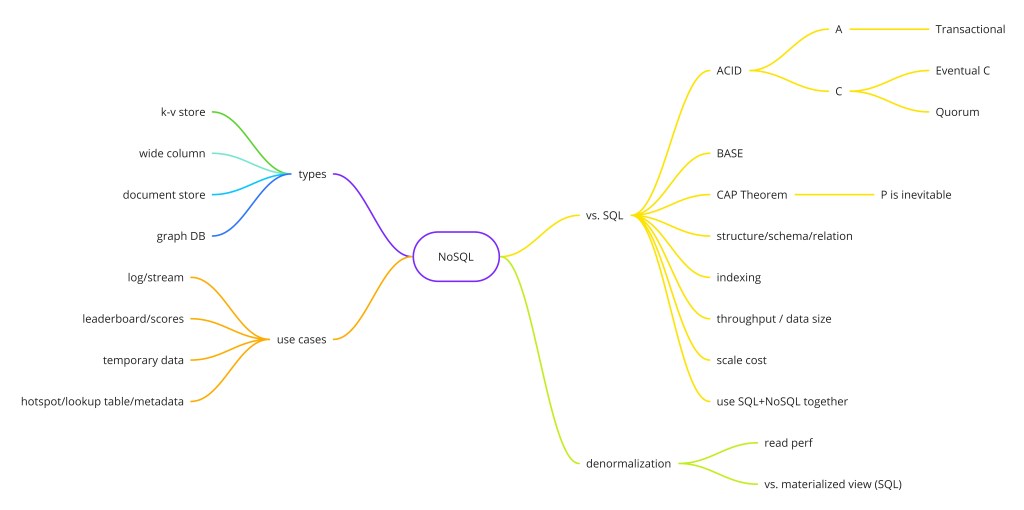
NoSQL ("Not Only SQL") is a broad category of database systems that abandon the relational table model in exchange for flexible schemas, horizontal scalability, and data models tuned for specific access patterns. They emerged as web-scale companies ran into the limits of relational databases under massive read/write throughput and rapidly evolving schemas. Google published Bigtable in 2006, Amazon published Dynamo in 2007, and an industry was born. Today NoSQL encompasses four fundamentally different data models — key-value, document, column-family, and graph — each solving a different class of problem. Understanding which model fits which workload, and why, is what separates a senior engineer's storage decisions from a junior one's coin-flip.
- Key-value — O(1) reads/writes by exact key; no schema, no queries; ideal for sessions, caching, rate limiting.
- Document — self-describing JSON/BSON; flexible schema, nested objects without joins; ideal for user profiles, catalogs.
- Column-family — rows keyed by row key, columns grouped by family stored together; ideal for time-series and high-write analytics workloads.
- Graph — native traversal of nodes and edges; ideal for social graphs, recommendations, fraud detection.
- CAP theorem — partition tolerance is mandatory; the real choice is CP (HBase, ZooKeeper) vs AP (Cassandra, DynamoDB in eventual mode).
- Default to SQL; reach for NoSQL only when you have a specific bottleneck that a specialized data model addresses.
NoSQL databases trade relational features (joins, strict ACID) for schema flexibility and horizontal scale. Pick the right type for your data model: document for nested objects, key-value for high-throughput lookups, column-family for time-series and analytics, graph for relationship traversal. The CAP theorem dictates that you must choose between consistency and availability during a network partition.
The Four NoSQL Categories
Key-Value Stores — The Speed Layer
The simplest data model: every value is stored under a unique key. Reads and writes are O(1) by key — literally a hash table lookup. There is no query language, no schema, and no relationships — just raw speed for exact lookups. The value itself is completely opaque to the store; it can be a string, a serialized object, a binary blob, or a counter. The database does not interpret it.
- Examples: Redis, DynamoDB (in KV mode), Memcached
- Best for: Session storage, cache layers, rate limiting counters, feature flags, leaderboards (with Redis sorted sets), distributed locks
- Limitation: Can only access data by exact key; no range scans without additional infrastructure; no secondary indexes unless the database adds them as a separate feature layer
Redis deserves special attention because it goes far beyond a simple KV store. Its data structures — strings, lists, sets, sorted sets, hashes, streams, and HyperLogLogs — let you implement sophisticated patterns like sliding-window rate limiters (ZRANGEBYSCORE on timestamps), pub/sub fanout, leaderboards (ZADD/ZRANK), and distributed locks via the SET key value NX PX ttl atomic conditional set. The key insight is that Redis executes all operations atomically in a single-threaded event loop, which eliminates the concurrency bugs that plague multi-threaded in-process caches.
# session storage with TTL
SET session:abc123 '{"userId":42,"role":"admin"}' EX 3600

# rate limiter: sliding window of 100 req/min per user
ZADD ratelimit:user42 1716550000.123 "req:a1b2"
ZREMRANGEBYSCORE ratelimit:user42 -inf 1716549940.000  # prune old entries
ZCARD ratelimit:user42                                    # count remaining in window

# distributed lock — atomic compare-and-set
SET lock:order-42 "owner-xyz" NX PX 30000  # only succeeds if key does not exist
Document Stores — The Schema-Flexibility Layer
Data is stored as self-describing documents (usually JSON or BSON). A document can contain nested objects and arrays, representing a complete entity without joins. The schema is flexible — different documents in the same collection can have different fields. This is not a weakness; it is a deliberate design choice. When your data model is genuinely heterogeneous (a product catalog where a laptop has CPU/RAM specs and a T-shirt has size/color variants), forcing everything into a normalized relational schema produces either a forest of nullable columns or the dreaded entity-attribute-value anti-pattern.
- Examples: MongoDB, Couchbase, Firestore
- Best for: User profiles, product catalogs, content management, any domain where the data is naturally hierarchical and the schema evolves frequently
- Limitation: Denormalized data means updates must be applied in multiple places; multi-document transactions are possible (MongoDB 4.0+ supports them) but expensive — they exist as a safety net, not the primary pattern
// MongoDB: insert and query a document
await db.collection('users').insertOne({
  _id: 'u-123',
  name: 'Alice',
  email: '[email protected]',
  address: { city: 'Seattle', zip: '98101' },  // nested object, no join needed
  tags: ['admin', 'beta']
});

const user = await db.collection('users').findOne(
  { 'address.city': 'Seattle' }   // query on nested field
);

// DynamoDB: single-table design pattern — all entity types in one table
// PK = "USER#alice"   SK = "PROFILE"           → user record
// PK = "USER#alice"   SK = "ORDER#2024-01-15"  → order record
// Enables single-query fetch of user + recent orders
const result = await ddb.query({
  TableName: 'AppTable',
  KeyConditionExpression: 'PK = :pk AND begins_with(SK, :prefix)',
  ExpressionAttributeValues: { ':pk': 'USER#alice', ':prefix': 'ORDER#' }
});
DynamoDB deserves its own mention here. Although marketed as a KV store, its composite key model (partition key + sort key) with GSIs and LSIs makes it a powerful document store for access-pattern-driven design. The single-table design pattern — storing all entity types in one table and co-locating related records via sort key prefix — lets you satisfy multiple access patterns in a single query, eliminating joins entirely at the cost of upfront modeling rigor.
Column-Family Stores — The Write-Scale Layer
Data is organized into rows identified by a row key, with columns grouped into column families. Columns within a family are stored together on disk, making it extremely efficient to read a large number of rows for a small set of columns — the classic analytics access pattern. Rows can have different columns, and new columns can be added without a schema migration. The key design insight: the primary key (in Cassandra, this is the partition key + clustering key) completely determines where data lives and what queries are efficient. You design tables around your query patterns, not around normalized entities.
- Examples: Apache Cassandra, HBase, Google Bigtable, ScyllaDB
- Best for: Time-series data (IoT sensors, metrics), event logs, leaderboards, write-heavy workloads like click-streams and user activity feeds
- Limitation: Query patterns must be modeled into the table design — you effectively denormalize around your queries; ad-hoc queries across different partition keys require full scans or secondary indexes, which are expensive
-- Cassandra: time-series sensor readings
-- Partition key: sensor_id (one partition = one sensor's data)
-- Clustering key: ts DESC (newest first within partition)
CREATE TABLE sensor_readings (
  sensor_id   UUID,
  ts          TIMESTAMP,
  value       DOUBLE,
  unit        TEXT,
  PRIMARY KEY (sensor_id, ts)
) WITH CLUSTERING ORDER BY (ts DESC);

-- Fetching last 100 readings for a sensor: single partition, no scatter
SELECT * FROM sensor_readings
WHERE sensor_id = 550e8400-e29b-41d4-a716-446655440000
LIMIT 100;

-- Cassandra write path: writes go to a commit log + memtable
-- then are periodically flushed to immutable SSTables on disk
-- → O(1) writes regardless of data volume
Cassandra's write path explains why it can sustain millions of writes per second: every write appends to an in-memory memtable and a sequential commit log, then the memtable is periodically flushed to an immutable SSTable. There are no in-place updates, no locking, no index maintenance at write time. The cost is paid at compaction time. This LSM-tree architecture (Log-Structured Merge-tree) is also used by RocksDB, LevelDB, and HBase — it is the fundamental reason column-family stores dominate write-heavy workloads.
Graph Databases — The Relationship Layer
Data is modeled as nodes (entities) and edges (relationships), with properties on both. Graph traversal — "find all friends of friends who live in NYC who also purchased product X" — is a native first-class operation, achieved without expensive multi-level joins. In a relational database, the same query requires multiple self-joins on a friendship table, and performance degrades polynomially with depth. In a graph database, each node directly stores pointers to its adjacent edges — traversal is O(degree) per hop regardless of total graph size.
- Examples: Neo4j, Amazon Neptune, ArangoDB, TigerGraph
- Best for: Social networks, recommendation engines, fraud detection (transaction graphs), knowledge graphs, network topology
- Limitation: Poor fit for bulk tabular data; horizontal sharding is harder than other NoSQL types because cutting a graph across partitions causes cross-shard traversal overhead; most graph DBs are best run on a single beefy node or a small cluster
// Neo4j Cypher: find 2nd-degree connections who are not already friends
MATCH (me:Person {id: 'alice'})-[:FRIENDS_WITH]->(friend)
                                 -[:FRIENDS_WITH]->(fof)
WHERE fof.id <> 'alice'
  AND NOT (me)-[:FRIENDS_WITH]->(fof)
RETURN fof.name, count(*) AS mutual_friends
ORDER BY mutual_friends DESC
LIMIT 10;

// Fraud detection: find shared identifiers between accounts
MATCH (a:Account)-[:USES]->(device:Device)<-[:USES]-(b:Account)
WHERE a.id <> b.id
RETURN a.id, b.id, device.fingerprint AS shared_device
CAP Theorem — The Distributed Systems Constraint
The CAP theorem, proved by Eric Brewer and formalized by Gilbert and Lynch, states that a distributed data store can only guarantee two of the following three properties simultaneously:
| Property | Meaning |
|---|---|
| Consistency (C) | Every read returns the most recent write or an error. All nodes see the same data at the same time. This is linearizability — a strong safety guarantee. |
| Availability (A) | Every request receives a non-error response, even if it may not be the most recent data. The system never refuses to serve. |
| Partition Tolerance (P) | The system continues to operate even if network partitions prevent some nodes from communicating. Messages can be lost or delayed between nodes. |
Network partitions are inevitable in any distributed system — a switch fails, a rack loses power, a cross-datacenter link degrades. So P is effectively mandatory. The real choice is between CP (sacrifice availability during a partition — return an error rather than stale data; HBase, ZooKeeper) and AP (sacrifice consistency — serve stale data rather than erroring out; Cassandra, DynamoDB in eventual-consistency mode). Most NoSQL databases let you tune this per-operation through consistency levels.
CAP only describes behavior during a network partition. PACELC extends it: even when there is no partition, there is still a tradeoff between Latency and Consistency. DynamoDB's "eventually consistent reads" are faster because they can serve from any replica; "strongly consistent reads" must route to the primary and wait for it to confirm no newer write exists. Real production systems are tuned on the PACELC axis far more often than the CAP axis, because partitions are rare but the latency/consistency tradeoff is constant.
Consistency Models in Depth
CAP's binary "C or A" framing is too coarse for production decisions. Real systems offer a spectrum of consistency guarantees, and understanding them lets you pick the right level per operation rather than per database:
- Linearizability (Strong Consistency) — every operation appears to execute atomically at a single point in time. Any read after a write returns that write. The safest, most expensive model. Used for financial ledgers, inventory counts. In Cassandra:
QUORUMreads withQUORUMwrites (more than half of replicas must respond). - Causal Consistency — if operation A causally precedes B (you wrote a post, then its reply was written), any read that sees B also sees A. Captures the happens-before relationship without requiring global ordering. Used in collaboration tools (Google Docs internal model). More available than linearizability, more correct than eventual consistency.
- Eventual Consistency — if no new writes happen, all replicas will eventually converge to the same value. No timing guarantee. Reads may return stale data. Suitable for social media likes, DNS, caches. In Cassandra:
ONEconsistency level means only one replica needs to respond — maximum throughput, maximum staleness risk. - Read-Your-Writes — a user always sees their own writes, even if other users may see stale data. Critical for any interactive UI — if you post a comment and immediately refresh, it should be visible. Achieved in Cassandra by routing the read to the same coordinator or using sticky sessions.
- Monotonic Reads — once a client reads value X, subsequent reads never return something older than X. Prevents the "ghost update" experience where a value appears to go backwards. Achieved by pinning reads to a replica.
-- Cassandra consistency levels for a 3-replica cluster
-- (RF=3, so QUORUM = 2 replicas must respond)

-- Strong consistency: W=QUORUM + R=QUORUM guarantees no stale reads
INSERT INTO orders (id, status) VALUES (42, 'PAID') USING CONSISTENCY QUORUM;
SELECT * FROM orders WHERE id = 42 CONSISTENCY QUORUM;

-- Maximum throughput: W=ANY + R=ONE — fastest but stalest
INSERT INTO page_views (url, ts) VALUES ('/home', now()) USING CONSISTENCY ANY;
SELECT count FROM page_view_totals WHERE url = '/home' CONSISTENCY ONE;
BASE vs. ACID — The Correctness Tradeoff
Relational databases are defined by ACID guarantees. NoSQL databases typically offer BASE semantics instead. Understanding this tradeoff is fundamental to choosing a storage layer:
| Property | ACID (SQL) | BASE (NoSQL) |
|---|---|---|
| Atomicity | All operations in a transaction succeed or all fail — no partial state | Single-entity operations are atomic; multi-entity operations may leave partial state visible |
| Consistency | Database moves from one valid state to another; constraints enforced | Basically Available — the system makes progress even with failures |
| Isolation | Concurrent transactions appear to execute serially | Soft state — data may change over time without an explicit write (TTL expiry, compaction) |
| Durability | Committed data survives crashes (WAL/journal) | Eventually Consistent — replicas converge without requiring synchronous agreement |
The practical consequence: use SQL and ACID for any domain where partial writes cause semantic errors — financial ledgers, inventory counts, order records. Use BASE semantics for domains where temporary inconsistency is acceptable — social feeds, read caches, analytics counters, recommendation scores. The mistake engineers make is assuming all their data falls into one category. In a real system, you almost always need both: a relational database for transactional truth, and one or more NoSQL stores for specific high-throughput or high-scale workloads.
Data Modeling Approaches
Document Store Modeling — Embed vs. Reference
The central design decision in document stores is whether to embed related data inside a document or reference it with a foreign-key equivalent. The rule of thumb follows the "one-to-squiggly" guideline: if the related entity has bounded cardinality and is always accessed with the parent, embed it. If it has unbounded cardinality or is sometimes accessed independently, reference it.
- Embed: A blog post embedding its tags, a product embedding its variant list, a user embedding their most recent address — all bounded, always read together.
- Reference: A blog post's comments (unbounded growth), a user's full order history (accessed independently), a product's seller (accessed independently) — unbounded or independently accessed.
The antipattern: embedding arrays that grow without bound. An order document embedding every comment about it will eventually hit MongoDB's 16 MB document size limit and slow down every read of that order even when comments aren't needed. Detect this by asking: "Does this array grow forever?" If yes, reference instead.
Column-Family Modeling — Design Tables Around Queries
In Cassandra you do not normalize data and then write queries. You write your queries first, then design tables to serve exactly those queries. Each table is a denormalized projection of your data optimized for one specific access pattern. A "user's activity feed" and "all activities of type X" require two separate tables in Cassandra, both populated on every write — a write amplification tradeoff that buys O(1) reads on known patterns.
-- Query 1: "show me user alice's feed, newest first"
CREATE TABLE user_feed_by_user (
  user_id     UUID,
  created_at  TIMESTAMP,
  activity_id UUID,
  type        TEXT,
  payload     TEXT,
  PRIMARY KEY (user_id, created_at, activity_id)
) WITH CLUSTERING ORDER BY (created_at DESC);

-- Query 2: "show all 'purchase' events globally, newest first"
CREATE TABLE activities_by_type (
  type        TEXT,
  created_at  TIMESTAMP,
  user_id     UUID,
  payload     TEXT,
  PRIMARY KEY (type, created_at)
) WITH CLUSTERING ORDER BY (created_at DESC);

-- On write: populate BOTH tables in the application
Representative Products Deep Dive
DynamoDB — Managed Scale at Any Cost
DynamoDB is AWS's fully managed, serverless NoSQL database. Its defining properties: single-digit millisecond latency at any scale, automatic sharding, and a pricing model based on provisioned or on-demand read/write capacity units. Its design philosophy — strongly opinionated about access patterns — forces upfront modeling discipline that pays off at scale. Global tables provide multi-region active-active replication with conflict resolution. DynamoDB Streams can feed CDC pipelines. The tradeoffs: complex queries are impossible without multiple tables and application-side joins; secondary indexes (GSI) are eventually consistent; cross-partition transactions exist (via TransactWriteItems) but are expensive and limited to 100 items.
MongoDB — The Document Generalist
MongoDB is the most widely deployed document database. Its aggregation pipeline — a sequence of stages including $match, $group, $lookup (server-side join), $unwind, and $project — covers analytics use cases that would require multiple queries in pure KV stores. Change Streams enable CDC-style pipelines. Atlas Search provides Lucene-powered full-text search on top of document collections. The tradeoffs: schema-less collections can become "schemaless chaos" if discipline is not applied via application-level validation or JSON Schema constraints; multi-document ACID transactions are available but should be the exception, not the rule; horizontal sharding requires explicit shard key planning and is operationally complex.
Cassandra — Write-Scale Champion
Cassandra was built by Facebook to power the inbox search feature, then open-sourced and adopted by Netflix, Apple, and Discord (who use it to store billions of messages). Its leaderless, peer-to-peer architecture (no primary node, no single point of failure) means it can absorb node failures and even datacenter outages without downtime. The consistent hashing ring distributes partitions across nodes, and the virtual node (vnode) concept spreads each physical node's token ranges to ensure even distribution even with heterogeneous hardware. Discord's famous "Cassandra migration" post documented how they moved from Cassandra to ScyllaDB (a C++ reimplementation with better JVM-free performance) — worth reading for the operational reality of column-family stores at scale.
Neo4j — The Graph Standard
Neo4j uses a native graph storage format where each node directly stores pointers to its adjacent edges, eliminating the index lookups that relational databases need for joins. Its Cypher query language is arguably more readable than SQL for relationship-heavy queries. The practical ceiling: Neo4j Community Edition is single-node; the Enterprise clustering model works well up to tens of billions of nodes and edges but sharding a property graph across machines remains a hard research problem. For truly massive graphs (Facebook's social graph), custom in-house solutions or purpose-built systems like JanusGraph on top of Cassandra/HBase are used.
CAP in Practice: NoSQL Product Placement
| Database | Type | CAP Position | Default Consistency |
|---|---|---|---|
| Redis (cluster) | KV | CP — primary holds writes; replicas may lag | Strong on primary; async replica |
| DynamoDB | KV / Document | AP (default) / CP (strong reads) | Eventual; opt-in strong |
| MongoDB | Document | CP (primary election) | Primary read by default; tunable |
| Cassandra | Column-family | AP (default) / CP (QUORUM) | Eventual; tunable per operation |
| HBase | Column-family | CP — writes blocked during region server failure | Strong (single region server owns range) |
| Neo4j | Graph | CP (single-primary writes) | Strong on primary; read replicas async |
NoSQL vs. SQL: When to Choose Which
| Scenario | Prefer SQL | Prefer NoSQL |
|---|---|---|
| Schema | Stable, well-defined relationships | Rapidly evolving or highly variable per entity |
| Transactions | Multi-table ACID required (finance, orders) | Single-entity updates sufficient; BASE acceptable |
| Query patterns | Flexible, ad-hoc SQL queries across entities | Known, repetitive access patterns designed upfront |
| Scale | Moderate — vertical scaling + read replicas | Massive — horizontal write scaling needed (millions/sec) |
| Consistency | Strong consistency required everywhere | Eventual consistency acceptable for most reads |
| Data shape | Tabular, normalized, relational | Hierarchical, graph-like, or time-series |
When Not to Use NoSQL
The hype cycle around NoSQL led many teams to abandon SQL prematurely. Here are the scenarios where NoSQL is the wrong choice:
- Complex multi-entity transactions — if a business operation touches multiple entity types and must be all-or-nothing (e.g., transfer $100 between two bank accounts and log the transaction), SQL's native ACID transactions are simpler, safer, and more performant than orchestrating distributed Sagas across multiple NoSQL stores.
- Heavy ad-hoc analytics — a Cassandra table designed for "user's recent orders" cannot answer "all orders placed between $50 and $100 in California last month" without a painful secondary index or full scan. SQL's query planner handles this elegantly.
- Strong relational constraints — foreign key enforcement, cascading deletes, and referential integrity are first-class SQL features. NoSQL stores give you none of these; you must enforce them in application code, where they are less reliable.
- Small to medium datasets with complex queries — Postgres with proper indexing handles hundreds of millions of rows comfortably. Reaching for Cassandra for a dataset that could live in a well-tuned Postgres instance adds operational complexity for no gain.
- Rapidly changing access patterns — if your query patterns evolve frequently, Cassandra's "design tables around queries" philosophy turns into a migration nightmare. SQL lets you add indexes later; Cassandra requires new tables.
Production systems at scale almost never use a single database type. A typical architecture: PostgreSQL for the transactional core (orders, accounts, users), MongoDB for flexible catalogs and content, Cassandra or DynamoDB for high-write event streams and time-series, Redis for caching and real-time counters, and Elasticsearch for full-text search. Each NoSQL store was added to solve a specific bottleneck, not to replace the relational core.
Performance and Scaling Patterns
Horizontal Sharding in NoSQL
Most NoSQL databases handle sharding automatically or semi-automatically. Understanding the mechanics matters when things go wrong. In Cassandra, consistent hashing distributes partition keys across the ring — but a poorly chosen partition key creates hot partitions where one node absorbs a disproportionate share of traffic. The cardinal rule: partition keys should have high cardinality and evenly distributed write load. Using a low-cardinality key (like "country code") as a partition key in Cassandra creates at most a few hundred partitions, leaving most nodes idle during peak.
In DynamoDB, hot partitions manifest as "ProvisionedThroughputExceededException" errors on specific keys. The mitigation is partition key sharding: append a random suffix (1–N) to the key, distribute writes across suffixed variants, and scatter-gather reads across all variants. Ugly but effective for pathological workloads like a global like counter on a viral post.
Replication and Conflict Resolution
Multi-replica stores face the write-conflict problem: two writes to the same key on different replicas before they sync. The resolution strategies, from simplest to most correct:
- Last-Write-Wins (LWW) — whichever write has the later timestamp wins. Used by Cassandra by default. Risk: clock skew means a write made 10ms later on a machine with a slow clock can be silently dropped. Acceptable for eventually-consistent data like user preferences, unacceptable for financial records.
- Multi-Value / Sibling Resolution — Riak (and some DynamoDB configurations) store both conflicting values and return them both to the client, which must merge them explicitly. Correct but complex — the client must implement merge logic.
- CRDTs (Conflict-free Replicated Data Types) — data structures mathematically guaranteed to merge without conflicts: G-Counters (grow-only), PN-Counters (increment/decrement), LWW-Element-Sets. Redis and Riak support CRDTs natively for specific use cases like distributed counters and sets.
NoSQL is not a replacement for relational databases — it is a set of specialized tools. Start with SQL; it handles most use cases well. Reach for NoSQL when you have a specific bottleneck: key-value for cache-speed lookups, document for flexible hierarchical data, column-family for high-write time-series, graph for deep relationship traversal. Model your data around your access patterns, understand the consistency level you're running at, and be deliberate about where you accept BASE over ACID. The best engineers use both in the same system.
Explain CAP theorem and what "P is mandatory" means. In any distributed system, network partitions will occur — so you cannot sacrifice P. The real tradeoff is CP (return an error or block during partition to stay consistent, e.g. HBase) vs AP (return possibly stale data to stay available, e.g. Cassandra). PACELC extends this: even without a partition, there is a constant latency/consistency tradeoff that matters far more day-to-day.
When would you choose column-family over document stores? When your write throughput is very high (millions/sec), your read patterns are known upfront, and you can afford to design tables around queries. Cassandra's LSM-tree write path makes writes O(1) regardless of data volume — document stores pay random-write costs at high volume.
Why can't you just use NoSQL for everything? NoSQL trades multi-table ACID transactions and flexible ad-hoc queries for scale and schema flexibility. If your domain has complex relationships and you need joins or cross-entity transactions, SQL is almost always simpler, safer, and operationally cheaper. Adding NoSQL prematurely adds operational complexity without a bottleneck to solve.
What is eventual consistency and when is it dangerous? Eventual consistency means replicas will converge over time, but reads may return stale data in the interim. It is dangerous for inventory counts (two threads both reading 1 and writing 0, leading to negative stock), financial balances, and anything where a stale read leads to a real-world action. Use strong consistency (QUORUM in Cassandra, strongly consistent reads in DynamoDB) for these cases — at higher latency cost.
What is the single-table design pattern in DynamoDB? Storing all entity types in one table and using composite sort keys (e.g. ORDER#2024-01, PROFILE) to co-locate related records so multiple entity types can be fetched in a single query without joins. It requires upfront access-pattern analysis but delivers O(1) reads for all modeled patterns.