Sharding is a technique for horizontally partitioning a database across multiple independent nodes, each called a shard, so that the dataset and the write load are distributed rather than concentrated on a single machine. When a single database server can no longer handle the volume of data or query throughput — and vertical scaling (bigger CPU, more RAM) has hit its ceiling — sharding is the next step. But sharding is not a free lunch: it trades a simple, strongly-consistent single-node model for a distributed system that makes cross-shard queries, transactions, and schema changes dramatically harder. Understanding when and how to shard — and which of the three core strategies to use — is one of the most consequential architectural decisions you will make.
This guide covers the full sharding decision space: horizontal vs vertical partitioning, all three sharding strategies in depth, the consistent hashing algorithm and why virtual nodes matter, shard key selection criteria, hotspot management, resharding with minimal disruption, cross-shard query handling, distributed transactions, and how sharding relates to replication. By the end you will have the vocabulary and mental models to make confident sharding decisions — and to articulate the tradeoffs clearly in a system design interview.
- Hash-based sharding gives even distribution but breaks range queries and requires full data migration when node count changes — unless you use consistent hashing.
- Range-based sharding enables efficient range scans but risks write hotspots on sequential keys like timestamps or auto-increment IDs.
- Directory-based sharding offers maximum flexibility at the cost of a high-availability lookup service on the critical path.
- Consistent hashing minimizes data movement to ~k/n keys when adding one node; virtual nodes smooth out uneven distribution.
- Shard key design is the most consequential decision — high cardinality, even write distribution, aligned with query patterns.
- Cross-shard joins must be done in the application layer (fetch + merge in memory) — avoid them by designing the shard key around your access patterns.
- Sharding and replication are orthogonal — each shard should itself be replicated for HA; you need both, not one or the other.
Sharding splits data across multiple database nodes by a shard key. Hash-based sharding gives even distribution; range-based sharding enables efficient range scans; directory-based sharding offers maximum flexibility. Consistent hashing minimizes data movement when resharding. The cost is real complexity: cross-shard queries, joins, and transactions require significant engineering effort. Shard only after exhausting vertical scaling, read replicas, and caching.
Before You Shard: The Scaling Ladder
Sharding is an expensive operational commitment. Before reaching for it, exhaust the options on the scaling ladder in order — each step adds less complexity than sharding:
- Vertical scaling — give the primary more CPU, RAM, and faster storage. Straightforward, but bounded by the largest commercially available instance type. A modern cloud instance can carry 192 vCPUs and 3 TB of RAM, handling hundreds of thousands of queries per second — most workloads never need to go beyond this.
- Read replicas — route read traffic to replicas; concentrate writes on the primary. Typically a 5–10× effective read capacity multiplier for read-heavy workloads (90:1 or higher read:write ratios). The primary still bottlenecks on writes.
- Caching — a Redis cache absorbing 95% of read traffic means your database only sees 5% of the full load. The effective capacity gain is enormous and requires no data architecture change.
- Functional decomposition (vertical partitioning) — split different business domains into separate databases, each running on its own server. The orders database, the catalog database, and the user database each scale independently without any single-table row-level splitting.
- Sharding (horizontal partitioning) — when a single table is too large or too hot for one server even after the above steps, split its rows across multiple shards.
A single PostgreSQL primary with replicas and a Redis cache can comfortably handle 100,000 reads/sec and 10,000 writes/sec. At 1,000,000 reads/sec or 100,000 writes/sec, you start to need sharding on the write path. Most startups never reach that scale. Shard when the pain is real, not when the architecture diagram looks cooler.
Vertical vs. Horizontal Partitioning
The word "partitioning" means different things depending on whether you split along the column axis or the row axis. Understanding the distinction matters because they solve different problems and are often used together.
| Dimension | Vertical Partitioning | Horizontal Partitioning (Sharding) |
|---|---|---|
| What is split | Columns — different tables/columns on different servers (functional decomposition) | Rows — the same table spread across multiple nodes |
| Scale limit | Bounded by the number of domain boundaries you can draw | Scales horizontally with node count — theoretically unbounded |
| Complexity introduced | Cross-service API calls instead of joins; service boundary design | Cross-shard queries, distributed transactions, resharding ops |
| Use case | Microservice decomposition, separating read-heavy from write-heavy columns | A single table exceeding the capacity of one server (users, events, messages) |
| Examples | User service DB, Order service DB, Product service DB | Users 1–10M on shard 1, Users 10M–20M on shard 2, ... |
Vertical partitioning (functional decomposition) is essentially what microservices do: each service owns its database, and the services communicate over APIs rather than via SQL joins. This is often the right first move because it eliminates cross-domain joins, allows independent scaling, and maps cleanly to team ownership — without any of the row-level complexity of horizontal sharding.
Horizontal sharding kicks in when a single service's table grows beyond what one server handles. The canonical examples: a social platform with 2 billion users, a payment system processing 100 million transactions per day, a messaging system storing 1 trillion messages. No vertical decomposition resolves these — the table itself must be split across machines.
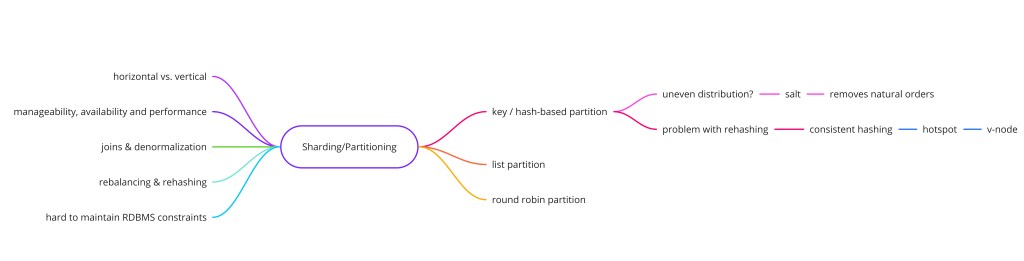
The Three Sharding Strategies
Hash-Based Sharding
Apply a hash function to the shard key and compute shard_id = hash(key) % num_shards to determine which shard holds a given row. The hash function distributes values uniformly regardless of the key's natural ordering, so data and write load are spread evenly across all shards.
def get_shard(user_id: int, num_shards: int) -> int:
    # consistent hash across shards — uniform distribution
    return hash(user_id) % num_shards

# user_id=1234567 with 8 shards → shard 3
# all data for user 1234567 lives on shard 3
# range query "users WHERE id BETWEEN 1M AND 2M" → must query ALL 8 shards- Pro: Uniform distribution — no single shard becomes disproportionately large unless the key space itself is skewed. Even write load across all shards.
- Con: Range queries require a scatter-gather fan-out to all shards and a merge in the application layer. Adding or removing a shard changes
num_shardsand remaps almost every key — a full data migration affecting(N-1)/N * total_datarows. - Best for: Workloads where queries always include the shard key (point lookups by user_id, order_id) and range scans are rare or routed to a separate analytics copy.
Range-Based Sharding
Partition rows into contiguous ranges of the shard key — e.g., user IDs 1–1,000,000 on shard 1, 1,000,001–2,000,000 on shard 2. The shard boundaries are explicitly defined in a routing table that maps each range to a shard.
- Pro: Range queries targeting a contiguous key range hit only the relevant shard(s) — no scatter-gather needed for common temporal or sequential queries. Easy to reason about data placement. Efficient for time-series data where queries frequently target recent windows.
- Con: Hotspot risk — the most critical failure mode. If recent data is the most active (as it almost always is with timestamps or auto-increment IDs), the highest-range shard (containing the newest data) bears nearly all write load while older shards are mostly cold. This completely negates the write throughput gains of sharding.
- Best for: Time-partitioned archival data where old data is cold and queries frequently target specific date windows. Not appropriate as the primary strategy for active write workloads unless you pre-shard to distribute the "hot" range.
Avoid using timestamps or sequential auto-increment IDs as the range shard key for active write workloads. Instead, use a compound key that combines a hash prefix with the timestamp: shard = crc32(user_id) % 16 determines the initial shard, and within that shard data is stored in time order. This gives range-query efficiency within a shard while distributing writes across all shards.
Directory-Based Sharding
A centralized lookup table (the "directory") explicitly maps each key (or key range) to its target shard. Every database request first queries the directory to find the correct shard, then queries that shard directly. The directory itself must be highly available and extremely low-latency since it is on the critical path of every database operation.
- Pro: Maximum flexibility — any key can be remapped to any shard at any time without changing the hashing or range logic. Allows gradual, surgical data migration: move specific hot tenants or accounts to dedicated shards without resharding everything. Handles tenant-level isolation requirements cleanly (multi-tenant SaaS where each enterprise customer gets their own shard).
- Con: The directory is a single point of failure and a potential performance bottleneck; it must be replicated (typically via strong-consistency consensus like Raft), cached aggressively, and treated with the same reliability rigor as the primary database. Adds a latency floor to every query (mitigated by caching the directory locally).
- Best for: Multi-tenant platforms, scenarios requiring irregular or policy-driven data placement, and gradual resharding operations where surgical key-by-key migration is preferred over bulk data movement.
| Strategy | Distribution | Range Queries | Resharding Cost | Flexibility |
|---|---|---|---|---|
| Hash-based | Uniform | Scatter-gather all shards | High (remaps ~all keys) | Low (fixed algorithm) |
| Range-based | Uneven (hotspot risk) | Single or few shards | Medium (split ranges) | Medium (ranges adjustable) |
| Directory-based | Configurable | Depends on mapping | Low (update mapping) | High (arbitrary placement) |
| Consistent hashing | Uniform with vnodes | Scatter-gather | Low (~k/n keys move) | Medium |
Consistent Hashing: The Algorithm in Depth
Standard modulo hash sharding has a catastrophic resharding problem: adding one node to an 8-node cluster changes the modulus from 8 to 9, invalidating 7/8 ≈ 88% of all key-to-shard mappings. Every one of those keys must be migrated to its new shard. This is prohibitively expensive for a live production system. Consistent hashing solves this elegantly.
The ring abstraction
Consistent hashing maps both nodes and keys onto a logical ring of integers (typically the full MD5 or SHA-1 hash space: 0 to 2128–1). Each node is placed at a position on the ring determined by hashing its identifier. Each key is placed at a position determined by hashing the key itself. A key is owned by the nearest node clockwise from its position.
When a node is added, it is placed at a new position on the ring and claims only the key range between itself and its counterclockwise neighbor. All other key assignments are undisturbed. When a node is removed, its key range passes to its clockwise successor. In both cases, only ~k/n keys move — a fraction of the total dataset proportional to the newly added or removed capacity.
import hashlib
from sortedcontainers import SortedDict

class ConsistentHashRing:
    def __init__(self, virtual_nodes=150):
        self.ring = SortedDict()          # sorted by hash position
        self.vnodes = virtual_nodes

    def _hash(self, key: str) -> int:
        return int(hashlib.md5(key.encode()).hexdigest(), 16)

    def add_node(self, node: str):
        for i in range(self.vnodes):
            h = self._hash(f"{node}#vn{i}")
            self.ring[h] = node               # 150 virtual nodes per physical node

    def remove_node(self, node: str):
        for i in range(self.vnodes):
            h = self._hash(f"{node}#vn{i}")
            del self.ring[h]

    def get_node(self, key: str) -> str:
        if not self.ring:
            raise ValueError("Ring is empty")
        h = self._hash(key)
        idx = self.ring.bisect_right(h) % len(self.ring)
        return self.ring.peekitem(idx)[1]   # clockwise nearest node
Virtual nodes: why 150?
With a small number of physical nodes (say, 3), the probability that the hash function places them evenly around the ring is low — you might end up with one node owning 60% of the key space and another owning 15%. Virtual nodes solve this by assigning each physical node multiple positions on the ring (150 is the Cassandra default). With 150 virtual nodes per physical node, the law of large numbers kicks in and load balances to within a few percentage points of ideal. The tradeoff is memory — the ring table grows by a factor of the virtual node count, but even at 1000 virtual nodes with 100 physical nodes, the ring table is only 100,000 entries, which is trivially small.
Virtual nodes also simplify heterogeneous clusters: a node with twice the memory and CPU capacity can be assigned 300 virtual nodes instead of 150, causing it to own ~twice the key space and bear twice the traffic — without any special-casing in the routing logic.
Shard Key Design: The Most Consequential Decision
The shard key is the column (or combination of columns) that determines which shard holds a given row. A bad shard key creates hotspots, forces scatter-gather on common queries, or breaks application-level join patterns. Once data is sharded, changing the shard key is extremely disruptive — it requires a full table reshuffle across shards. Get this right before you write the first row.
Properties of a good shard key
- High cardinality — enough distinct values to spread data across all shards without collisions. A boolean column (active/inactive) has cardinality 2 — catastrophically bad as a shard key. A UUID or a high-cardinality ID column works well.
- Even write distribution — the distribution of writes across the key's value space should be uniform. Monotonically increasing keys (auto-increment IDs, timestamps) fail this for hash sharding because the "current" value is always the highest, concentrating writes. Use a hash or UUID-derived key instead.
- Aligned with access patterns — the single most important property. If your most common query is "get all orders for user X," sharding orders by
user_idmeans that query hits exactly one shard. Sharding byorder_idscatters a user's orders across all shards and forces a fan-out on every user-facing request. - Stable — if the shard key value changes (e.g., a user changes their email, which you naively used as the shard key), the row needs to move to a different shard. Immutable keys (internal UUIDs, auto-increment IDs generated at insert time) avoid this problem entirely.
Real-world shard key examples
- Social platform users table — shard by
user_id(hash). All per-user reads are single-shard. Cross-user analytics fan out to all shards and are redirected to a data warehouse. - E-commerce orders table — shard by
user_id(notorder_id!) so "my orders" reads are single-shard. Merchant-side "all orders for product X" must fan out — acceptable if routed to a separate analytics replica. - Time-series IoT events table — shard by
device_id(hash) so all events from one device are co-located and time-window queries on a single device are single-shard. Sharding by timestamp alone concentrates all current writes on one shard. - Multi-tenant SaaS — shard by
tenant_idusing a directory so large enterprise customers can be isolated to dedicated shards and small customers are co-located on shared shards.
Hotspots and Resharding
Hotspots: when a shard becomes a bottleneck
A hotspot occurs when a disproportionate fraction of reads or writes routes to a single shard. This can happen for three reasons:
- Skewed key distribution — if the shard key's value distribution is not uniform (e.g., most users are in one geographic region), hash sharding will not distribute evenly.
- Hot entities — a celebrity user on a social platform might have 50 million followers all generating events on the same shard. No shard key design fully prevents entity-level hotspots; the mitigation is to denormalize (fan-out events to follower shards) or to add a cache layer in front of the hot shard.
- Time-based writes with range sharding — the "current" range shard absorbs all writes. Mitigation: use hash sharding for write distribution and range sharding only in analytics/archival tiers.
Resharding: adding capacity without a full migration
As data grows, individual shards fill up and performance degrades. Resharding — splitting existing shards or adding new ones — is one of the most operationally intensive tasks in a sharded system. The techniques, roughly from least to most disruptive:
- Read replica promotion — if one shard is write-hot but read-heavy, promote a replica to a co-primary that handles reads independently. This buys time but does not actually split the data.
- Shard splitting — divide one overloaded shard into two. For range sharding: update the boundary in the routing table and migrate the upper half of rows to the new shard. For consistent hashing: add a new node to the ring; only the key range between the new node and its predecessor migrates.
- Online schema change tooling — when resharding requires schema changes across all shards, use
gh-ost(GitHub's Online Schema Change) orpt-online-schema-changeto make changes without blocking production writes. - Double-write + backfill pattern — write to both the old and new shard layout simultaneously while a background job copies existing data from old to new. Once the backfill is complete and verified, cut over reads to the new layout and stop double-writes. This allows zero-downtime resharding at the cost of temporary write amplification.
# Online resharding: double-write + backfill pattern

Phase 1 — Dual-write (no downtime):
  All writes → old shard AND new shard layout
  Reads still served from old shard

Phase 2 — Backfill (background):
  Copy all existing rows from old → new layout
  Track progress by primary key range
  Verify checksums per batch

Phase 3 — Cutover (brief read pause or zero-downtime):
  Verify new shard is fully consistent with old
  Switch reads to new shard layout
  Stop dual-writes to old layout

Phase 4 — Cleanup:
  Drop old shard data after validation period
Cross-Shard Queries and Transactions
Cross-shard queries: the scatter-gather problem
Any query that does not include the shard key in its WHERE clause must be broadcast to all shards (scatter), and the results merged in the application layer (gather). This is called a scatter-gather fan-out, and it is the most common performance problem in sharded systems:
- Query latency is bounded by the slowest shard, not the average. If 1 of 16 shards is slow, all fan-out queries wait for it.
- Fan-out queries generate
Nqueries whereNis the shard count. At 64 shards, a single user-facing request generates 64 database queries. This caps the effective concurrent user capacity. - Result merging in the application layer (sorting, deduplication, aggregation) adds CPU and memory pressure to the app tier.
Mitigations:
- Design the shard key to align with your most common query pattern — this is the only real fix. Accept that other query patterns will be more expensive.
- Route analytical / cross-shard queries to a separate data warehouse or OLAP system (Redshift, BigQuery, ClickHouse) that holds denormalized copies of the data. Never run analytics directly against OLTP shards.
- Denormalize aggressively — store redundant copies of data on multiple shards to enable local reads. For example, store a copy of the user's name on every order shard so "orders with user name" queries do not need a cross-shard user join.
- Maintain a global secondary index — a separate index shard that maps non-shard-key fields to shard locations. Adds write complexity (must keep the index in sync) but avoids scatter-gather for indexed lookups.
Cross-shard transactions: the hardest problem
ACID transactions spanning multiple shards are one of the hardest problems in distributed systems. The two standard approaches, and their tradeoffs:
- Two-phase commit (2PC) — a coordinator asks all participant shards to prepare (Phase 1) and then commit (Phase 2). Guarantees atomicity. The problem: the coordinator holds locks on all participant shards between Phase 1 and Phase 2. If the coordinator crashes between phases, the shards are left in an indeterminate state, blocking indefinitely (the "blocking problem"). Also creates a performance bottleneck: all transactions with cross-shard scope serialize through the coordinator.
- Saga pattern — decompose the transaction into a sequence of local single-shard transactions, each publishing an event that triggers the next step. Compensating transactions undo completed steps on failure. Sagas are eventually consistent, not atomically consistent — there is a window where the system is in a partially-committed state. Appropriate for business transactions (e-commerce checkout, money transfer) but not for low-level data integrity constraints.
The cleanest way to avoid cross-shard transactions is to design your sharding so that every critical transaction touches only one shard. This usually means co-locating related data that participates in the same transaction. For an e-commerce platform, sharding both orders and cart data by user_id means the checkout transaction (which reads the cart and writes an order) is single-shard for a given user.
Sharding vs. Replication: Orthogonal Concerns
Sharding and replication are frequently confused but solve entirely different problems:
| Dimension | Sharding | Replication |
|---|---|---|
| What it solves | Write throughput and dataset size beyond a single node | Read throughput, high availability, and fault tolerance |
| Data distribution | Each row exists on exactly one shard (no duplication) | Each row exists on multiple replicas (full duplication) |
| Node failure impact | One shard lost = that subset of data unavailable | Primary lost = replica promotes; no data loss |
| Read scalability | N shards × 1 primary each = N parallel write+read primaries | Fan reads to replicas; primary handles writes only |
| Are they exclusive? | No — combine them. Each shard should itself be replicated: a 4-shard cluster with 3 replicas each = 12 total nodes. | |
A production sharded system always combines both: sharding for write scalability and dataset partitioning, replication for read scalability and high availability. Without replication, losing a single shard node makes an entire partition of your data unavailable. Without sharding, a single replicated primary becomes a write bottleneck as data grows.
Schema Changes Across Shards
DDL operations (adding a column, adding an index, changing a data type) must be applied to every shard — often 8, 16, or 64 identical schema mutations that each need to run without locking production traffic. The operational discipline required:
- Online schema change tools —
gh-ost(GitHub) andpt-online-schema-change(Percona) apply DDL changes via a shadow-table-and-trigger approach that never takes a full table lock. Essential for tables with millions of rows. - Backward-compatible migrations — always make schema changes in two phases: first deploy code that can handle both the old and new schema, then apply the DDL, then remove the old-schema-handling code. This allows rollback at any step without schema inconsistency.
- Shard-by-shard rollout — apply the DDL to one shard at a time and monitor for errors before proceeding. A bad migration on one shard can be stopped before it affects the others.
- Automation is non-negotiable — manually SSHing into 64 shards to run
ALTER TABLEis not a process. Build schema migration tooling that applies changes to all shards systematically, with per-shard success/failure tracking and automatic rollback.
Real-World Sharding Architectures
Vitess (YouTube / PlanetScale)
Vitess is a sharding middleware layer built around MySQL that adds connection pooling, query routing, and horizontal sharding on top of standard MySQL. It was originally built by YouTube to handle billions of rows of video metadata. Vitess introduces a concept called VShards (logical shards) that can be remapped to physical MySQL instances without application code changes. The routing layer handles scatter-gather, cross-shard aggregation, and shard-aware SQL rewriting automatically. PlanetScale offers Vitess as a managed service.
Cassandra's built-in sharding
Cassandra is a distributed database that uses consistent hashing with virtual nodes internally — sharding is built into the storage engine, not bolted on at the application layer. Data is partitioned by a partition key, and rows with the same partition key are co-located (these are called wide rows or clustering columns). A well-designed Cassandra data model aligns the partition key with the most common access pattern and keeps partition sizes manageable (under ~100 MB). Cassandra's strengths — linear write scalability, no master node, tunable consistency — make it well-suited to high-write, known-access-pattern workloads like messaging systems, IoT time series, and activity feeds.
DynamoDB's transparent sharding
DynamoDB shards automatically based on your provisioned or on-demand capacity settings — the shard topology is invisible to the application. You design a partition key (hash key) and an optional sort key (range key), and DynamoDB routes requests to the correct internal shard. The constraint is that a single partition key cannot exceed 10 GB of storage or 3,000 RCUs / 1,000 WCUs — violating this creates a hot partition that throttles requests.
Shard only when you have exhausted vertical scaling, read replicas, and caching — the added operational complexity is real and permanent. When you do shard, invest heavily in shard key design: high cardinality, even write distribution, and alignment with your most common query pattern. Use consistent hashing with virtual nodes to minimize data movement during topology changes. Accept that cross-shard queries and transactions are expensive and design your data model to make them rare. And remember: each shard needs its own replication — sharding and replication are orthogonal, complementary tools.
Hash vs range sharding — when to pick each? Hash for even write distribution across many keys (user_id, device_id); range when you need efficient time-window or contiguous key scans and can tolerate hotspot risk (or you route writes through a hash prefix to distribute them).
Why is consistent hashing better than modulo sharding? Adding a node with modulo hashing remaps ~(N-1)/N of all keys (nearly everything); consistent hashing moves only ~k/n keys to the new node, minimizing data migration and allowing live resharding with minimal disruption.
What makes a bad shard key? Low cardinality (boolean, enum), monotonically increasing values (timestamps, auto-increment) with hash sharding, or keys misaligned with query patterns — all create hotspots or force expensive scatter-gather fan-outs.
How do you handle a cross-shard transaction? Prefer co-locating related transactional data on the same shard by design. When unavoidable, use the Saga pattern (eventual consistency with compensating actions) over 2PC (which creates blocking and coordinator bottlenecks).
What is the difference between sharding and replication? Sharding distributes different rows across nodes for write scalability; replication copies the same rows to multiple nodes for read scalability and HA. Production systems need both — each shard is itself replicated.