Reliable, Scalable & Maintainable

Chapter 1 sets the vocabulary for the entire book. Kleppmann argues that modern applications are data-intensive rather than compute-intensive — the real challenges are the volume, complexity, and speed of data. Three properties define a good data system: it must be reliable, scalable, and maintainable. This chapter unpacks each one with concrete examples.

Original Notes

The handwritten study notes this chapter summary is based on:

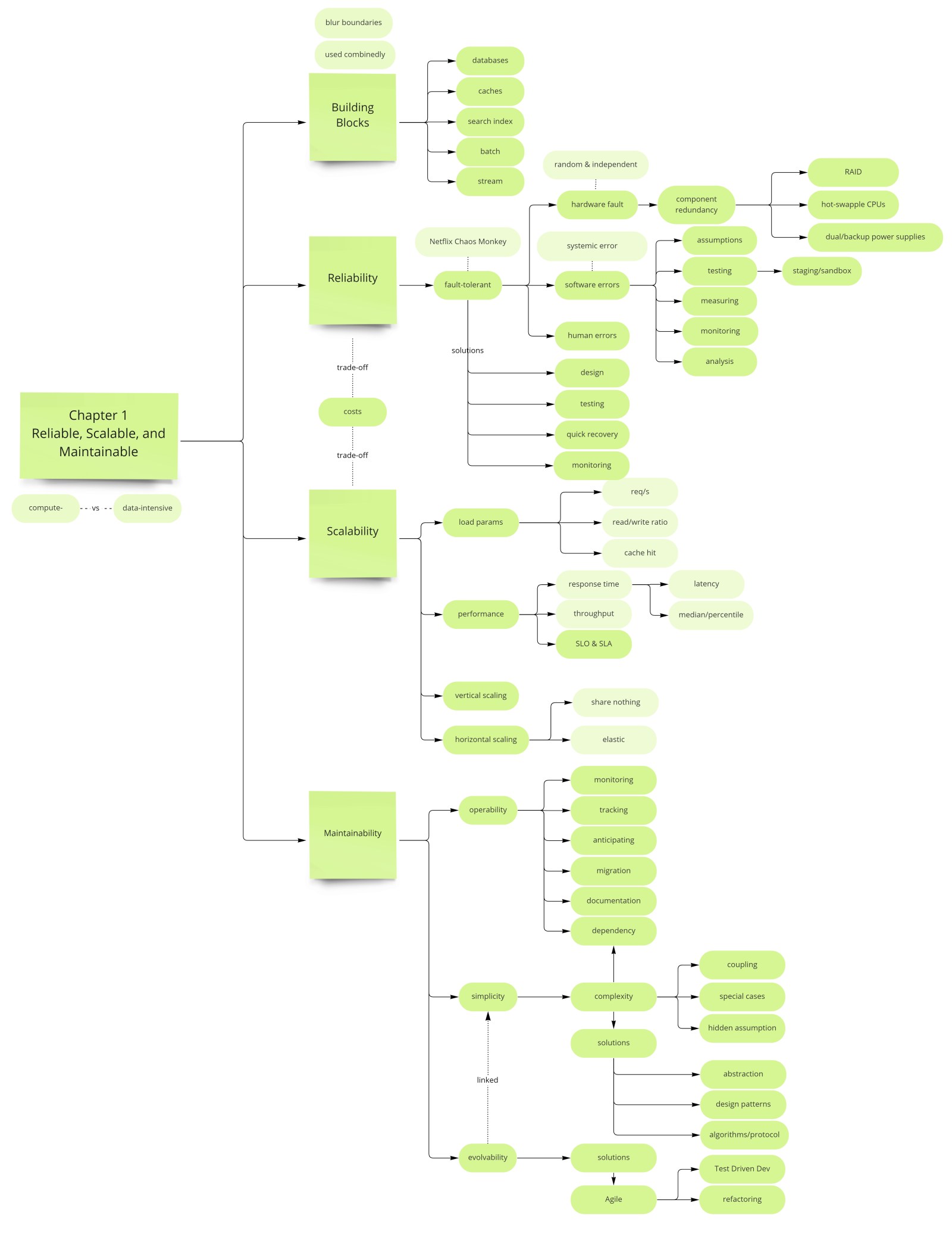
Reliability

A reliable system continues to work correctly even when things go wrong. Kleppmann draws a sharp distinction between a fault and a failure: a fault is when one component deviates from its spec; a failure is when the system as a whole stops providing the required service. The goal of fault-tolerant systems is to prevent faults from escalating into failures. Note that it can make sense to deliberately trigger faults — the chaos engineering practice pioneered by Netflix's Chaos Monkey — precisely to prove that the fault-tolerance machinery actually works and hasn't quietly atrophied.

Hardware Faults

Hard disks crash, RAM develops bad bits, power grids flicker, and someone unplugs the wrong cable. The mean time to failure of a single hard disk is roughly 10–50 years, but in a cluster of 10,000 disks you expect to lose a disk every day. Until recently the standard response was hardware-level redundancy — RAID arrays, dual power supplies, hot-swap CPUs, diesel generators. These were sufficient when a single machine was the unit of deployment.

As data volumes and compute requirements grew, applications began running on large numbers of commodity machines. Cloud platforms (AWS, GCP, Azure) explicitly do not guarantee single-machine reliability; instead they design for virtual machine preemption and node loss. The modern answer is multi-machine redundancy in software: replicated databases, stateless application servers behind load balancers, and rolling upgrades that take nodes out of rotation one at a time so the system keeps serving traffic throughout. Hardware faults remain relevant, but they are now handled by architecture, not just hardware spend.

Software Faults (Systematic Faults)

Software bugs are far more dangerous than hardware faults precisely because of that correlation. A bug in one node's binary is likely present on every other node too, meaning it can take down an entire cluster simultaneously — something a disk failure never does. Kleppmann gives several canonical examples of systematic faults in the wild:

• A software bug that crashes every instance simultaneously when a specific unusual input is provided (e.g. a malformed date, an integer overflow).
• A runaway process that slowly consumes all CPU or memory until the node becomes unresponsive.
• A service that responds slowly to requests, causing cascading timeouts in dependent services that pile up connections and exhaust their own thread pools — a failure mode that propagates through a microservice graph.
• A dependency that starts returning corrupted or unexpected responses after a version upgrade, corrupting data in callers silently.

There is no silver bullet. The mitigations are engineering discipline: careful reasoning about assumptions and interactions at design time, thorough automated testing at unit, integration, and end-to-end levels, process isolation to limit blast radius, crash-and-restart policies (let it fail fast rather than limp along corrupting data), and continuous monitoring with alerting on unexpected invariant violations. Systematic faults often lie dormant for months until a specific condition triggers them, which is why production monitoring of invariants matters even when everything seems fine.

Human Errors

Post-mortem analyses of large-scale internet service outages consistently identify operator mistakes as the single leading cause — misconfigured deployments, accidental deletion, wrong database connection string, schema migration applied to the wrong environment. Humans are both the designers and operators of these systems, and they are inevitably fallible. Good system design accepts this and reduces the blast radius:

• Well-designed abstractions that make wrong things hard to do — an API surface that requires an explicit destructive-action flag rather than silently accepting dangerous commands.
• Sandbox and staging environments where engineers can experiment and make mistakes without touching production data.
• Automated testing at every level — unit tests, integration tests, and end-to-end tests — so that a misconfiguration is caught before it ships.
• Easy and fast rollback — a deployment that can be reverted in under two minutes limits the window of a human-caused outage.
• Detailed monitoring, metrics, and logs — if an operator makes a mistake, you want to detect it in seconds, not hours. Monitoring also provides early warning of anomalies that can be corrected before they escalate.
• Good operational playbooks and runbooks — on-call engineers should not be relying on tribal knowledge at 3 AM when a novel failure occurs.

Fault Tolerance Design Patterns

Understanding the fault taxonomy guides which design patterns to reach for. Hardware faults call for replication and redundancy. Software faults call for isolation boundaries, circuit breakers, and gradual rollouts. Human errors call for process guardrails and observability. Across all three categories, the guiding principle is the same: expect faults to occur, design the system to detect and contain them, and make recovery fast.

Fault Type	Characteristic	Primary Mitigations
Hardware faults	Independent failures; statistically predictable at scale	RAID, replication, multi-AZ, rolling upgrades
Software faults	Correlated; can take down all nodes at once	Testing, process isolation, gradual rollout, monitoring
Human errors	Leading cause of outages; hard to eliminate	Sandboxes, abstractions, fast rollback, runbooks

Scalability

Scalability is not a one-dimensional label you apply to a system. The question is always more specific: "If the system grows in this particular way, how do we cope?" Growing by 10× users is different from growing by 10× data volume, and different again from growing by 10× request rate with the same user count. You must first describe your load precisely using load parameters, then measure how performance changes as those parameters increase, and only then decide how to handle growth. Skipping straight to "we need to horizontally scale" without defining load is a red flag in a system design interview.

Describing Load: Load Parameters

A load parameter is a number that meaningfully characterizes the load on your system. The right choice of parameter depends on the system's architecture and the nature of its bottleneck. Examples across different systems:

• Web server: requests per second, and the distribution of request types (read vs write, cached vs uncached).
• Database: read/write ratio; number of concurrent connections; size of the working set relative to available memory.
• Chat application: number of simultaneously active users; message fanout per message (how many recipients per sender).
• Search engine: query rate; index size; freshness requirements (how soon new documents must appear).
• Cache: hit rate — a cache hit rate of 99% versus 95% is a 5× difference in DB load, not a 4% difference.

The Twitter Fan-Out Case Study

Kleppmann uses Twitter's home timeline as the definitive fan-out example, because it cleanly illustrates how the distribution of a load parameter matters more than its average value. The problem: when you open Twitter, you see a merged timeline of everyone you follow. There are two fundamentally different ways to serve this.

Approach 1 — Pull on read (query at request time): When a user requests their home timeline, the system looks up all accounts they follow, fetches each account's recent tweets, sorts and merges the results by timestamp, and returns the page. Write a tweet → just insert one row into a tweets table. Simple. The problem is read cost: if you follow 400 accounts, timeline generation requires 400 lookups plus a merge sort. At Twitter's scale (300M monthly active users at the time of the book's writing), this is hundreds of millions of expensive fan-out reads per second.

Approach 2 — Fan-out on write (push at tweet time): When a user posts a tweet, the system immediately pushes that tweet into the pre-computed home timeline cache of every follower. Reading a timeline becomes a single cache lookup — extremely cheap. The cost is at write time: posting one tweet triggers N cache writes, where N is the poster's follower count. For most users this is fine. For a celebrity with 30 million followers, a single tweet triggers 30 million cache writes — a massive write amplification spike that can overwhelm the system.

Twitter's actual solution is a hybrid: fan-out on write for the vast majority of users (where follower counts are modest), and pull-on-read for a small set of high-follower accounts (celebrities, news outlets). Most timelines are pre-computed; a small number of celebrity tweets are stitched in at read time. The critical insight: the correct load parameter to reason about is not "average tweet rate" but the distribution of followers per user — specifically the long tail of high-follower accounts that makes naive fan-out on write infeasible.

Describing Performance: Response Time vs Latency

Before measuring performance, it is worth clarifying terminology that is often conflated. Latency is the time a request spends waiting to be processed — the time it sits in a queue before the system picks it up. Response time is what the client measures from sending the request to receiving the full response; it includes network time, queuing time, and processing time. In practice, "latency" is used loosely to mean response time, and Kleppmann uses the terms interchangeably in conversational context while being precise when it matters.

For online services, response time is the performance metric that matters to users. For batch systems, throughput (records processed per second or per hour) is usually more relevant. These require different optimization strategies: minimizing response time often means prioritizing individual request processing; maximizing throughput often means batching work and saturating resources fully, accepting higher per-request latency.

Why the Mean Is the Wrong Metric

Mean (average) response time is almost always the wrong metric. It is sensitive to the arithmetic of skewed distributions: a small number of very slow requests inflate the mean dramatically, but they disappear into it statistically — you cannot tell whether the mean of 200 ms represents a system where every request takes 200 ms or a system where 90% take 50 ms and 10% take 1.5 s. Both have the same mean. Only percentiles let you see the difference.

Percentile	Meaning	Why It Matters	Typical Use
p50 (median)	Half of requests are faster than this	Represents the typical user experience	Baseline health check
p95	95 of 100 requests are faster	Shows tail behavior without extreme outliers	Common SLO target
p99	99 of 100 requests are faster	Captures high-value user experience	SLA commitment to customers
p999	999 of 1000 requests are faster	The absolute worst non-anomaly experience	Amazon internal service targets

High percentile latencies — often called tail latency — matter disproportionately for two reasons. First, users with the slowest experience are often your most engaged and highest-value users: they have more data (longer history, more connections, more items in their shopping cart), so every query touches more rows and takes longer. Optimizing for the median while ignoring the tail is optimizing for the easy, low-value case. Second, modern applications make many backend calls in parallel to assemble a page; the end-to-end response time is bounded by the slowest of those calls, not the average. If just one in twenty backend calls is slow (a p95 event), and a page render requires 20 parallel calls, then on average every page render will be delayed by that p95 outlier.

Service level objectives (SLOs) and service level agreements (SLAs) are defined in percentiles for exactly this reason. A typical SLO might read: "p99 of user-facing read requests must be below 200 ms, measured over a rolling 5-minute window." An SLA is a contractual version of this, with penalty clauses for violation. Both are meaningless if stated in terms of averages.

Head-of-Line Blocking and Load Testing

Head-of-line blocking is a subtle but important amplifier of tail latency. Servers process requests concurrently, but only up to their thread pool or connection limit. When a small number of slow requests occupy those threads, subsequent requests queue up behind them and experience high latency even though the server itself is not overloaded on average. The slow requests are blocking the queue head, holding everything back. This effect means that even a p95 slowness on individual requests can produce much higher end-to-end latency at the page level, because multiple requests may hit the queue behind slow ones.

Measuring response time on the client side rather than only on the server side is essential for capturing head-of-line blocking. Server-side p99 of 50 ms can coexist with client-side p99 of 2 s if requests are queuing. When running load tests, sending requests at a fixed rate (not waiting for each to complete before sending the next) is critical — otherwise you only measure performance at low load rather than the behavior when the server is under genuine concurrent stress.

Approaches to Coping with Load

Once you have described load parameters and measured performance, you face the question of how to scale. The two fundamental strategies are vertical and horizontal scaling, but the real decision is more nuanced:

• Scaling up (vertical scaling) — move to a more powerful machine: more CPUs, more RAM, faster disk. The advantage is simplicity; you do not change the architecture. The disadvantage is that powerful machines are non-linearly more expensive than commodity ones, and there is a hard ceiling — you can only buy so much CPU on a single node. Vertical scaling works well for databases where shared-nothing horizontal partitioning is architecturally complex.
• Scaling out (horizontal scaling, shared-nothing) — distribute load across more commodity machines. Each machine owns a subset of data or handles a subset of requests. More complex to build and operate, but the ceiling is much higher and cost scales more linearly with load. Stateless services (e.g. HTTP API handlers) scale out naturally; stateful services (e.g. databases) require careful partitioning design.
• Elastic vs manual scaling — elastic systems detect load increases and automatically provision new instances (autoscaling in cloud environments). Manual scaling requires a human to judge when to add capacity. Elastic scaling is appropriate for highly variable load (e.g. a news site whose traffic spikes on breaking news); manual scaling is simpler and sufficient for systems with predictable, slowly-growing load.

The choice between vertical and horizontal scaling is not purely technical — it involves operational complexity, cost curves, and the nature of the workload. A system designed from day one as horizontally scalable is often over-engineered for a startup that could have run on a single Postgres instance for years. The pragmatic approach: start simple, identify actual bottlenecks with real data, and scale the specific bottleneck rather than speculating about future load.

Maintainability

The majority of the cost of software is not in its initial development but in ongoing maintenance: fixing bugs, keeping systems operational, investigating failures, adapting to new platforms, repaying technical debt, and adding new features. Engineers who maintain systems they did not originally build spend much of their time fighting complexity that was unnecessary and could have been avoided with better design choices upfront. Kleppmann identifies three design principles for maintainability, each targeting a different axis of ongoing cost.

Operability: Making Life Easy for Operations

Operations teams are responsible for keeping the system running 24/7. They are not the authors of the code — they are the people who get paged at 3 AM when something breaks. A system is operable if it helps them do their job efficiently and minimizes the cognitive load of routine tasks and incident response.

Concretely, good operability means:

• Visibility into runtime behavior — rich metrics exposed via Prometheus/StatsD, structured logs queryable in a log aggregation system (e.g. Elasticsearch, Splunk), and distributed traces that let an engineer see the full causal chain of a single request across dozens of services. Without observability, operations is guesswork.
• Standard tooling interfaces — a system that integrates with existing monitoring, deployment, and alerting frameworks requires no custom one-off tooling to operate. Operators should be able to apply skills and playbooks from other systems.
• No single-machine dependency — the system should tolerate rolling restarts, machine replacements, and patch application without taking the service down. This requires stateless application tiers and replicated stateful tiers.
• Good default behavior with overrides — safe defaults that work for 95% of situations, with explicit override mechanisms for the other 5%. Operators should never have to dig into source code to understand why the system is behaving unexpectedly.
• Predictable behavior — surprises are the enemy of on-call. A system that occasionally stalls for 30 seconds "for no apparent reason" (e.g. a stop-the-world GC pause, a background compaction job) is much harder to operate than one with predictable latency characteristics.
• Good documentation — architecture diagrams, runbooks for common failure modes, an explanation of every configuration knob and its effect. Documentation that is out of date is almost worse than none, because it creates false confidence.

Simplicity: Managing Complexity

Kleppmann is direct: managing complexity is the single biggest challenge in large-scale software development. Complexity is not just about the number of lines of code — it is about the cognitive load required to understand the system well enough to make a correct change. A complex system is one where every change requires understanding a large number of non-obvious interactions; where adding a feature in one place silently breaks something apparently unrelated; where every engineer maintains a private and slightly different mental model, leading to subtle bugs at the boundaries.

Kleppmann distinguishes two kinds of complexity. Essential complexity is inherent to the problem domain — a tax calculation engine handling the rules of every jurisdiction has irreducible complexity because the problem itself is complex. Accidental complexity is introduced by the implementation, not required by the problem — unnecessary state, tight coupling between unrelated components, confusing naming, deeply nested conditional logic, or an abstraction that leaks its internals at every use site. The goal is to minimize accidental complexity while accepting that essential complexity is unavoidable.

The primary tool for managing complexity is a good abstraction: a clean conceptual boundary that hides implementation detail behind a simple interface. SQL is Kleppmann's canonical example. Behind a SQL query is a complex B-tree structure, a buffer pool, a transaction log, a query optimizer, and a lock manager — none of which the SQL author needs to understand. The abstraction lets one clean concept (a table of rows, queried declaratively) be used in thousands of applications without each developer reinventing or needing to understand the storage layer. When abstractions are good, they significantly reduce the mental surface area every engineer must hold in their head.

Evolvability: Making Change Easy

Software requirements are not static. The business pivots, new regulations arrive, performance characteristics change, and features that seemed important turn out not to be used while unanticipated use cases emerge. A system that cannot be safely changed without heroic effort is a liability — it either ossifies as technical debt accumulates, or it gets rewritten at great expense. Evolvability (also called extensibility or modifiability) is the property of a system that makes change tractable.

At the small scale of individual files and functions, agile practices address evolvability: test-driven development ensures a safety net exists before refactoring; continuous refactoring keeps the local code structure from calcifying; short feedback loops catch regressions quickly. These are necessary but not sufficient for large systems.

At the architectural scale, evolvability requires design decisions that keep independent concerns separated. If adding a new feature requires understanding and modifying ten different services because they are all tightly coupled, the system is not evolvable. If adding a new encoding format for data requires updating every consumer simultaneously because there is no schema evolution mechanism, the system is not evolvable. This is why later chapters of DDIA focus so heavily on schema evolution strategies (Avro, Protocol Buffers, Thrift), backward/forward compatibility, and stream processing architectures that decouple data producers from consumers — all of these are tools for buying evolvability at the system design level.

Maintainability Pillar	Core Question	Key Tools and Practices
Operability	Can ops keep this running without heroic effort?	Metrics, logs, traces, runbooks, rolling deploys, predictable behavior
Simplicity	Can a new engineer understand this system quickly?	Good abstractions, minimal coupling, clean interfaces, avoid accidental complexity
Evolvability	Can we safely change this system over time?	Schema evolution, loose coupling, backward compatibility, TDD, refactoring culture

The Interplay of All Three Properties

Reliability, scalability, and maintainability are not independent — they interact and often trade off against each other. A system that prioritizes scalability by adding caching layers and asynchronous processing becomes harder to operate and reason about, reducing maintainability. A system that prioritizes reliability through extensive redundancy and fault-tolerant design becomes more complex and thus harder to evolve. The engineer's task is not to maximize any one property in isolation but to find the right balance for the problem at hand, given the team's size, the system's expected growth trajectory, and the cost of failure.

Kleppmann's framing — reliability, scalability, maintainability — is deliberately used as the organizing lens for the rest of DDIA. When he introduces a new technique (replication, partitioning, transactions, stream processing), he always returns to these three questions: does this help the system be more reliable, more scalable, or more maintainable? The answer is rarely "all three simultaneously" — each technique has a primary target and secondary costs, and understanding those costs is the mark of engineering maturity.