A map platform like Google Maps serves billions of users across wildly different use cases — turn-by-turn navigation, business discovery, satellite imagery, traffic-aware routing, and third-party integrations for apps like Uber. At 3 billion monthly active users and 10 million API partners, it is one of the most data-intensive and latency-sensitive systems in existence. The core challenge is not storing the world's road network — it is answering "what is the fastest route between two points right now?" in tens of milliseconds, for millions of concurrent users, while continuously integrating fresh traffic data from billions of location pings.
- Geohash encodes 2D → 1D — converts lat/lng to a sortable string, enabling efficient range queries on standard key-value stores (BigTable/DynamoDB/Cassandra).
- Pre-compute routes — Dijkstra is O((V+E)logV); too slow at 3B users. Store pre-computed routes between section nodes; only the final micro-segment is computed on-the-fly.
- Contraction Hierarchies — offline node-importance ranking lets query-time bidirectional Dijkstra skip low-importance nodes, achieving 1000× speedup over vanilla Dijkstra.
- WebSockets for navigation — bidirectional persistent connection; a WebSocket Manager maps user IDs to server:port for routing.
- At-most-once for location pings — GPS sent every 5s; one lost packet is acceptable, guaranteed delivery overhead is not.
- CDC → Elasticsearch — map changes flow through Kafka to keep the search index eventually consistent.
- Map tiles served from CDN — pre-rendered raster tiles keyed by zoom/x/y; the most cacheable objects in the system.
Pre-compute routes between sectional nodes and store them in a geohash-indexed key-value store (BigTable/DynamoDB/Cassandra). Use Contraction Hierarchies offline to make query-time routing 1000× faster than vanilla Dijkstra. Use WebSockets for real-time navigation. Feed user location pings (every 5s, at-most-once) into a message queue. Serve map tiles from CDN. Let CDC-driven Kafka keep the Elasticsearch search index current with map changes. Push ML-powered ETA refinement and hotspot prediction offline.
Step 1 — Clarify Requirements
A map platform is deceptively broad. Scoping it in an interview into a concrete surface is half the credit. State what you will cover and explicitly call out what you won't.
Functional
- Identify roads, places, and points of interest on a rendered map.
- Calculate accurate distance and ETA accounting for traffic, road conditions, and real-time incidents.
- Turn-by-turn navigation with live rerouting on deviation or new incidents.
- Nearby search: find restaurants, gas stations, hospitals within a radius.
- Map tile rendering at multiple zoom levels.
- Provide a pluggable API for third-party integration (ride-share, vehicle manufacturers, data providers).
Non-Functional
- Low latency — route queries must return in <100 ms p99; tile loads under 50 ms from CDN cache.
- High availability — navigation failures mid-trip are critical user experiences; target 99.99%.
- Massive scale — 3 billion monthly active users, 10 million API partners.
- Eventual consistency acceptable for map data — a newly added road appearing in search 30 seconds late is fine; a wrong route is not.
- Durability of map edits — user-submitted corrections must not be lost.
Distinguish between the read path (tiles, routing, search) and the write path (map edits, live traffic ingestion). They have very different consistency requirements and can be designed almost independently. Call this split out early — interviewers reward it.
Step 2 — Capacity Estimation
Google Maps serves roughly 1 billion daily active users (DAU). Let's build a back-of-the-envelope estimate for the three main traffic types: tile fetches, route requests, and location pings.
Map Tile Traffic
- Each map view loads ~10–20 tiles (a 3×3 or 4×4 grid around the viewport).
- 1B DAU × 20 sessions/day × 15 tiles/session = 300 billion tile fetches/day ≈ 3.5M tiles/sec.
- The vast majority are served from CDN edge caches — the origin tile server handles only cache misses (<1% of requests).
- Tile storage: the world has ~4.5 trillion tiles across all zoom levels; at ~20 KB per raster tile, that is roughly 90 PB of tile data — the reason tile storage uses distributed object stores (GCS/S3) and only hot zoom levels are fully pre-rendered.
Route Requests
- Assume 10% of DAU request a route per day: 100M route requests/day ≈ ~1,200 route QPS average, with a 5× peak → ~6,000 route QPS.
- Each route request may fan out to 3–5 alternative routes, so the routing engine handles ~30K sub-queries per second at peak.
Location Pings (Active Navigation)
- Assume 50M users are navigating simultaneously at peak (commute hours).
- Each navigator sends a GPS ping every 5 seconds: 50M / 5 = 10M location writes/sec.
- Each ping is ~100 bytes: 10M × 100B = ~1 GB/sec of inbound location data — must be absorbed by a horizontally partitioned message queue.
Map Data Storage
- Road network graph: ~50M nodes (intersections) × 200B + ~100M edges × 100B ≈ ~20 GB for the raw graph (fits in memory on a large machine, enabling in-memory routing).
- Place/POI data: ~500M places × ~500B ≈ ~250 GB in the place database.
- Traffic data: streaming, retained for 30 days → roughly ~10 TB of historical traffic at compressed storage.
Step 3 — API Design
Expose clean REST endpoints through the API gateway. The three most important surfaces for interview purposes are tile serving, routing, and nearby search.
# Map tiles — zoom/x/y follows the standard slippy map scheme
GET  /tiles/{zoom}/{x}/{y}.png
     → 200 image/png  (served from CDN edge, TTL ~7d)

# Route calculation
POST /api/route
     { origin: {lat, lng}, destination: {lat, lng},
       mode: "driving"|"walking"|"transit",
       alternatives: true }
     → { routes: [{ polyline, distance_m, duration_s, eta }] }

# Nearby search (radius in meters)
GET  /api/places/nearby?lat=37.7&lng=-122.4&radius=500&type=restaurant
     → { places: [{ place_id, name, lat, lng, rating }] }

# Geocoding (address → coordinates)
GET  /api/geocode?address=1600+Amphitheatre+Pkwy

# Reverse geocoding (coordinates → address)
GET  /api/reverse-geocode?lat=37.42&lng=-122.08

# Navigation session (WebSocket upgrade)
GET  /ws/navigate?route_id=abc123
     → WS stream: { type: "update", eta_s, next_maneuver, reroute? }
Two design choices worth calling out: the tile endpoint uses the slippy map (XYZ) scheme so that tile URLs are deterministic and maximally cacheable — the same tile URL can be cached globally without any query-string variance. The navigation endpoint upgrades to a WebSocket so the server can push ETA updates and rerouting instructions without the client polling.
Step 4 — Map Data: Ingestion and Storage
Initial map data is sourced from government municipal maps (e.g., USGS, Ordnance Survey), satellite imagery providers (Planet, Maxar), street-level imagery vehicles, and third-party geographic data providers. Continuous updates arrive via user-submitted feedback, business submissions, and ongoing satellite refreshes. OpenStreetMap volunteers contribute corrections at massive scale.
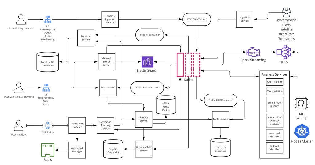
All map modifications are processed through Kafka via Change Data Capture (CDC), enabling downstream consumers — search indexers, route pre-computers, tile renderers, analytics services — to react to map changes asynchronously without coupling the ingestion path to downstream write latency.
Data Model: Road Network Graph
The road network is modeled as a directed weighted graph. Every intersection is a node; every road segment between two intersections is a directed edge with attributes including distance, speed limit, average travel time, road class (motorway, arterial, local), and turn restrictions.
CREATE TABLE nodes (
  node_id       BIGINT PRIMARY KEY,
  lat           DOUBLE NOT NULL,
  lng           DOUBLE NOT NULL,
  geohash       VARCHAR(12),          -- pre-computed, indexed
  node_type     VARCHAR(20)           -- intersection | endpoint | poi
);

CREATE TABLE edges (
  edge_id       BIGINT PRIMARY KEY,
  from_node     BIGINT REFERENCES nodes(node_id),
  to_node       BIGINT REFERENCES nodes(node_id),
  distance_m    INT   NOT NULL,
  speed_limit   SMALLINT,            -- km/h
  road_class    SMALLINT,            -- 0=motorway .. 5=local
  base_weight   FLOAT,               -- static travel time seconds
  current_weight FLOAT               -- traffic-adjusted, refreshed ~5 min
);

CREATE TABLE places (
  place_id      BIGINT PRIMARY KEY,
  name          VARCHAR(255),
  lat           DOUBLE,
  lng           DOUBLE,
  geohash       VARCHAR(12),
  category      VARCHAR(64),
  rating        FLOAT,
  address       TEXT
);
Step 5 — Spatial Indexing: Geohash, Quadtree, and S2
The core spatial indexing challenge is answering "give me all road nodes / places within this bounding box" efficiently at database scale. Three complementary structures power geospatial queries in modern map systems:
Geohash
Geohash encodes a 2D (lat, lng) coordinate into a 1D sortable Base32 string. Each additional character approximately quadruples the precision: a 6-character geohash covers ~1.2 km × 0.6 km; a 9-character hash covers ~5 m × 5 m. The key insight is that nearby locations share a common prefix — so a range scan on the geohash column retrieves spatially nearby records without any special spatial database extension. This makes it compatible with any key-value store (BigTable, DynamoDB, Cassandra) that supports efficient prefix queries.
-- Nearby places query using geohash prefix
FUNCTION nearby_places(lat, lng, radius_m):
  precision = geohash_precision_for_radius(radius_m)  -- e.g. 6 chars for 1km
  center_hash = geohash_encode(lat, lng, precision)
  neighbor_hashes = geohash_neighbors(center_hash)    -- 8 adjacent cells
  candidates = SELECT * FROM places
               WHERE geohash LIKE ANY(center_hash, neighbor_hashes)
  RETURN filter_by_haversine_distance(candidates, lat, lng, radius_m)
The neighbor query is critical: a search radius can straddle geohash cell boundaries, so you must always query the center cell plus its 8 immediate neighbors, then apply a precise Haversine distance filter to the candidates.
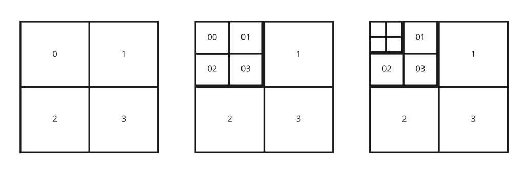
Quadtree
A quadtree recursively subdivides the map into four quadrants until each leaf cell contains fewer than a threshold number of objects (typically 50–100). It is ideal for dynamic density-adaptive indexing: a rural county and downtown Manhattan end up at very different subdivision depths. Quadtrees are used to power zoom-level-aware rendering — at low zoom, a node represents an entire region; at high zoom it resolves to an individual road or building. The quadtree is typically kept in memory on the tile servers and rebuilt periodically from the underlying database.
Google S2 Geometry
S2 maps the sphere onto the faces of a cube, then uses Hilbert curve indexing to produce a space-filling 1D cell hierarchy. Like geohash, S2 cells can be stored in any ordered key-value store; unlike geohash, S2 cells have more uniform area at each level and work correctly at the poles. Google Maps internally relies on S2 for many of its spatial operations — it is worth mentioning as the production-grade alternative to geohash if asked.
Step 6 — Map Tile Rendering and Delivery
Map tiles are the visual layer of the platform. A tile is a 256×256 (or 512×512 on retina) image representing a fixed geographic bounding box at a specific zoom level. The slippy map XYZ scheme defines tile coordinates: zoom level z, column x, row y — making every tile URL globally unique and deterministic, which is the key property enabling aggressive CDN caching.
Tile Generation Pipeline
- Vector data — the tile generator reads road, boundary, and POI data from the map database, renders it into raster images using a rendering engine (Mapnik or equivalent), and stores the results in distributed object storage (GCS/S3).
- Zoom level strategy — the full tile pyramid has ~4.5 trillion tiles. Only zoom levels 0–14 (global to city block) are pre-rendered in full; zoom levels 15–22 (building-scale) are rendered on demand and cached aggressively.
- Differential re-rendering — when map data changes (a new road, a renamed street), the CDC event triggers re-rendering of only the affected tiles by computing which XYZ cells intersect the modified geographic region. Bulk global re-render runs periodically as a batch job.
- CDN distribution — pre-rendered tiles are pushed to CDN edge nodes geographically close to users. A tile served from a CDN edge takes <5 ms; a cache miss that hits the origin object store takes ~50 ms. The cache hit rate for popular zoom levels exceeds 99%.
Serving pre-rendered raster tiles is the highest-leverage caching decision in a map system. A tile for downtown Manhattan gets requested millions of times per day — render it once, cache it everywhere. Vector tile streaming (sending raw geographic data for client-side rendering) reduces bandwidth and enables dynamic styling, but at the cost of client-side compute and reduced cacheability. Google Maps uses a hybrid: vector tiles for high zoom levels (street detail) and raster for lower zooms.
Step 7 — Routing Algorithm Deep Dive
Standard graph traversal (BFS) does not work for routing because road segments have variable weights (distance, speed limit, traffic). The correct algorithm for single-source shortest path is Dijkstra (or A* with a heuristic for faster convergence). However, running Dijkstra across the full global road graph at query time has time complexity of O((V+E)logV) — far too expensive for billions of concurrent users. The production answer is a layered pre-computation strategy.
Algorithm Comparison
| Algorithm | Complexity | Use case | Verdict |
|---|---|---|---|
| BFS | O(V+E) | Unweighted graphs | Wrong — ignores road weights |
| Dijkstra | O((V+E)logV) | Single-source shortest path | Correct but too slow at global scale |
| A* | O((V+E)logV) best-case faster | Heuristic-guided single-pair | Good for local routing, not global |
| Floyd-Warshall | O(V³) | All-pairs shortest paths | Offline pre-computation for small subgraphs only |
| Contraction Hierarchies | O(V log V) preprocessing; O(√V) query | Road networks | Production choice — 1000× faster than Dijkstra |
Contraction Hierarchies (CH)
Contraction Hierarchies is the dominant algorithm in production map routing. The core idea: assign each node an importance rank offline (based on edge difference, number of shortcuts needed, and road class), then iteratively "contract" the least-important nodes by replacing their incident edge pairs with direct shortcut edges that preserve shortest-path distances. The preprocessing produces a hierarchical graph where highway nodes have the highest ranks.
At query time, bidirectional Dijkstra runs simultaneously from source and destination, but each search only relaxes edges going upward in the hierarchy — skipping low-importance nodes entirely. This pruning reduces the search space from millions of nodes to thousands, delivering query times under 10 ms on continental-scale road networks.
-- CH bidirectional query (simplified)
FUNCTION ch_route(source, target):
  forward_dist  = {source: 0, all others: ∞}
  backward_dist = {target: 0, all others: ∞}
  forward_pq    = MinHeap([(0, source)])
  backward_pq   = MinHeap([(0, target)])
  best = ∞

  WHILE either queue non-empty:
    -- Expand from whichever direction has smaller tentative distance
    IF forward_pq.min() <= backward_pq.min():
      (d, u) = forward_pq.pop()
      FOR edge (u → v) WHERE rank(v) > rank(u):  -- upward only
        IF forward_dist[u] + w(u,v) < forward_dist[v]:
          forward_dist[v] = forward_dist[u] + w(u,v)
          forward_pq.push((forward_dist[v], v))
        best = min(best, forward_dist[v] + backward_dist[v])
    ELSE:
      -- Symmetric backward expansion
      ...
  RETURN best
Pre-Computation Strategy
Beyond CH, the system also sacrifices storage for speed at a geographic level: routes between sampled section boundary nodes (think: on-ramps and off-ramps for highway sections, or neighborhood entry points for urban areas) are fully pre-computed and stored in the key-value routing store. Navigation then resolves to a table lookup across sections rather than a live graph traversal for the bulk of the route. Only the first and last micro-segments (neighborhood-level) require on-the-fly Dijkstra/A*.
When a traffic incident causes a significant ETA change, the impact bubbles up recursively through the section hierarchy, updating only the affected route segments rather than recomputing globally. A change on a local road updates that road's section cache; only if the section's best-path changes does the update propagate to the next section tier.
Step 8 — Real-Time Navigation
Navigation sessions require bidirectional, low-latency communication between server and client — WebSockets are the right protocol here. A WebSocket Manager maintains a key-value mapping of connected users to their WebSocket server and port, enabling the Navigation Tracking Service to reach any active session regardless of which WebSocket server hosts it.
Three events trigger a navigation update:
- Route deviation — user strays from the planned path; recalculate using the pre-computed route cache from the new position.
- Significant ETA delay — a new incident on the route exceeds a threshold (e.g., +5 minutes); notify user and offer alternatives.
- Better route available — proactively reroute if a faster path opens up (e.g., traffic clears on a parallel highway).
User starts navigation
  → Navigation Service assigns route_id, opens WS connection
  → WebSocket Manager records: user_id → ws_server:port

Every 5 seconds:
  Client sends: { user_id, lat, lng, speed, heading }
    → Location Queue (Kafka, at-most-once)
      ├── Traffic Aggregator: update road segment weights
      └── Navigation Tracker: detect deviation / ETA change

On deviation detected:
  Navigation Tracker → Routing Service (CH query from new position)
    → Result pushed back via WebSocket Manager → client WS
      { type: "reroute", new_polyline, new_eta_s }
Step 9 — User Location Tracking
Active users transmit their GPS location every 5 seconds (when location sharing is enabled). These packets flow into a Kafka message queue that decouples producers from consumers. The delivery guarantee is at-most-once: a single lost location packet is acceptable because the next one arrives 5 seconds later, and the cost of guaranteed delivery (retransmission, ACKs, deduplication) would far outweigh the benefit for this use case.
The location stream serves multiple downstream consumers in parallel:
- Traffic Aggregator — aggregates speed readings across a road segment to compute real-time travel times; feeds back into the edge weight store that routing queries use.
- Navigation Tracker — per-user session state; detects deviations and triggers rerouting.
- Analysis Service — batch processing for ETA refinement, road discovery, and hotspot prediction.
- Ride-share / Third-party API consumers — external partners who subscribe to anonymized, aggregated traffic data.
Traffic Data Fusion
Raw GPS pings are noisy and sparse. The Traffic Aggregator applies a map-matching step: projecting the raw GPS coordinate onto the most likely road segment using Hidden Markov Models (the GPS reading is a "noisy observation" of the true position on the road network). Matched readings are then averaged over a 5-minute window per road segment to produce a reliable current travel time. These averages are written back to the current_weight field on the edges table, which the Contraction Hierarchy query engine reads at query time.
Step 10 — Search and Discovery
Place name search is powered by an Elasticsearch cluster supporting fuzzy matching and type-ahead. The index is populated from two streams: direct place name data and map CDC events. Map browsing displays nodes with priority-based filtering that adapts to zoom level — zooming out shows only major landmarks; zooming in reveals fine-grained detail.
Geocoding Pipeline
Geocoding (address string → lat/lng) is a multi-stage NLP pipeline:
- Parsing — tokenize the address into components (house number, street, city, postal code, country).
- Normalization — "St." → "Street", "Ave" → "Avenue"; handle abbreviations and international formats.
- Candidate retrieval — query Elasticsearch for matching street + city combinations using fuzzy matching to handle typos.
- Ranking — score candidates by match quality, popularity (how often this address is queried), and geographic context (prefer results near the user's current location).
- Interpolation — derive the house number position by linearly interpolating along the matched street segment.
Reverse geocoding (lat/lng → address) runs the pipeline in reverse: find the closest road segment using geohash lookup, then determine the nearest address via interpolation.
Step 11 — Scaling: Caching, Sharding, and CDN
Tile Caching
Map tiles are the single most cacheable object in the system. The cache hierarchy works outward from the client:
- Browser cache — tile images cached with long Cache-Control max-age (7 days); ~80% of tile requests are served from the browser cache on return visits.
- CDN edge — geographically distributed nodes; a tile for any given XYZ triple is the same for all users, so the CDN hit rate exceeds 99% for popular zoom levels.
- Origin object store — GCS/S3 serves the remaining cache misses; pre-rendered tiles are organized in a bucket hierarchy matching the XYZ tile scheme.
Routing Cache
Pre-computed section-to-section route results are stored in a distributed key-value store (Redis cluster or BigTable), keyed by (section_node_a, section_node_b, mode). A route request from San Francisco to Los Angeles resolves to a handful of section lookups rather than a live CH query. The cache is invalidated when traffic data changes the shortest-path cost for a given section pair beyond a threshold.
Database Sharding
- Node/edge graph — partitioned by geographic region (continent → country → state). Most routing queries are regional, so intra-region lookups stay on one shard. Cross-region routes join at section boundaries.
- Place data — sharded by geohash prefix, so "nearby search" queries land on a single shard or a small set of adjacent shards.
- Location ping stream — Kafka partitions by geohash cell, keeping pings for nearby road segments on the same partition for efficient aggregation.
Step 12 — Fault Tolerance
- Routing fallback — if the pre-computed route cache is unavailable, fall back to a live CH query against the in-memory graph; if that times out, fall back to a cached "last good" route. Never return an error when a stale route is better than nothing.
- CDN multi-origin — tile CDN is configured with two origin object store buckets in different regions; if the primary origin is unreachable, the CDN fails over to the secondary automatically.
- Navigation session continuity — WebSocket Manager state is stored in Redis with replication; if a WebSocket server crashes, the reconnecting client is assigned to a new server which re-fetches its session state from Redis within <1 second.
- Kafka replication — location ping topics are replicated across 3 brokers; consumer groups use offset commits so no ping is processed twice after a broker restart.
- Map data idempotency — each map edit carries a globally unique edit_id; idempotent write handlers ensure that a retried CDC event (e.g., after a consumer restart) does not apply the same road edit twice.
Step 13 — ML and Analysis Service
The Analysis Service consumes location and behavioral data to power several advanced features:
- ETA refinement — the base ETA from routing is computed from historical average speeds. The ML model adjusts it using real-time traffic speed, time-of-day patterns, weather, and historical trip duration percentiles for the specific O/D pair. The result is a probability distribution (e.g., "25 min with 80% confidence, 32 min at 95th percentile") rather than a point estimate.
- Hotspot prediction — forecasting congestion zones using temporal patterns (Friday evening at the bridge) and event data (concert ending times); surfaces alternative routes before congestion materializes.
- Road discovery — identifying unmapped roads or path changes through aggregate user travel patterns. If many users take a consistent off-graph path, the system flags it for human review and potential map update.
- User profiling — driving habits, typical speed patterns, home/office location prediction for proactive trip planning.
- Data source scoring — reliability weighting for user-submitted incidents vs. third-party providers vs. sensor data.
Key Tradeoffs
| Decision | Choice | Trade-off accepted |
|---|---|---|
| Route computation | Pre-compute + CH + store | Large storage and preprocessing cost; routes slightly stale until traffic cache refreshes (~5 min) |
| Location delivery | At-most-once (Kafka) | Single lost 5-second ping has negligible impact; saves substantial infrastructure complexity |
| Spatial indexing | Geohash (primary) + quadtree (rendering) | Geohash cell boundary edge cases require querying 9 neighbor cells; minor post-filter needed |
| Map data consistency | CDC eventual consistency | New road may take 30–60 sec to appear in search / routing; acceptable for map data |
| Tile strategy | Pre-rendered raster tiles | Re-render cost on map changes; less flexible styling than vector tiles |
| Traffic freshness | 5-minute aggregate windows | Real-time speed less accurate than per-second; prevents write amplification on edge weights |
Map systems live or die on their spatial indexing and pre-computation strategy. Geohash bridges 2D geography to 1D key-value lookups; Contraction Hierarchies make routing queries 1000× faster than Dijkstra at the cost of offline preprocessing; pre-rendered tiles make the most cacheable objects in the system nearly free to serve. Everything else — CDC pipelines, WebSocket navigation, at-most-once location pings, traffic fusion — is about keeping these pre-computed answers current and delivering them fast.
Why not run Dijkstra in real time for every route request? O((V+E)logV) across a global road graph is infeasible at 3B users — use Contraction Hierarchies offline to preprocess a hierarchy, then bidirectional Dijkstra at query time explores only a tiny fraction of nodes and returns in <10 ms.
Why geohash over a pure quadtree? Geohash encodes 2D coordinates into a 1D sortable string, enabling efficient range queries on standard key-value stores without special spatial index support. Quadtrees are better for zoom-adaptive rendering density.
Why at-most-once for location pings? A single lost 5-second GPS packet has negligible impact on navigation quality; the overhead of guaranteed delivery (retries, ACKs, deduplication) far outweighs the benefit at 10M writes/sec.
How do you handle stale routing when traffic changes? The traffic aggregator refreshes road segment weights on 5-minute windows; the pre-computed section cache is invalidated when the shortest-path cost changes beyond a threshold, triggering a targeted recompute for affected section pairs only.
How do map tiles stay fast? The XYZ slippy map scheme makes every tile URL deterministic, enabling near-100% CDN hit rates for popular zoom levels. Only cache misses touch the origin object store.